
NIFA Conservation Effects Assessment Project (CEAP)
Watershed Assessment Studies
Lessons Learned from the National Institute of Food and Agriculture (NIFA)-CEAP Synthesis Fact Sheet 7
Thirteen agricultural projects were funded by the USDA National Institute of Food and Agriculture (NIFA) and Natural Resource Conservation Service (NRCS) to evaluate the effects of agricultural conservation practices on spatial patterns and trends in water quality at the watershed scale. In some projects, participants also investigated how social and economic factors influence implementation and maintenance of practices. The 13 projects were conducted from 2004 to 2011 as part of the overall Conservation Effects Assessment Project (CEAP). The NIFA-CEAP projects were mainly retrospective; most conservation practices and water quality monitoring efforts were implemented through programs that occurred before the NIFACEAP projects began. By synthesizing the results of all these NIFA-CEAP projects, we explore lessons learned about identifying a watershed’s critical source areas in order to prioritize conservation practice implementation for better protection of water quality and lower costs.
National Institute of Food and Agriculture

National Resources Conservation Service
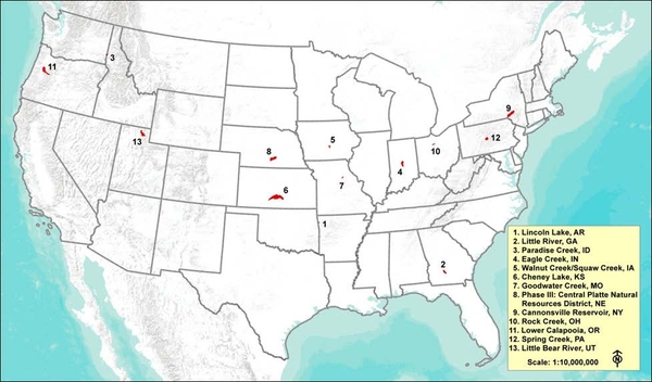
NIFA-CEAP watershed locations.
The Concept of Critical Source Areas (CSA)
Researchers have widely observed that a relatively small fraction of a watershed can generate a disproportionate amount of pollutant load, particularly phosphorus (P) and sediment (Pionke et al. 2000, Gburek et al. 2000, Yang and Weersink 2004). Simply put, the majority of a nonpoint source pollutant load can come from a minority of the watershed land. By identifying critical source areas (CSAs) in a watershed, we can prioritize conservation practices to better protect water quality and reduce costs. The CSA concept may not apply equally to all nonpoint source pollutants. Nitrogen issues, for example, can be spatially extensive where leaching coincides with excess nitrate in the soil profile over broad areas (Heathwaite et al. 2000).
Critical source areas occur where a pollutant source (such as a P source) in the landscape coincides with active hydrologic transport mechanisms. Research indicates that these areas pose a high risk for excessive pollutant export to surface waters. For example, in Oklahoma watersheds, White et al. (2009) reported that just 5% of the land area yielded 50% of the sediment load and 34% of the P load. And in a large Vermont river basin, about 74% of the annual nonpoint source P load was estimated to come from just 10% of the land area (Winchell et al. 2011).
Two factors help us to identify a CSA: pollutant sources and transport potential. Pollutant sources in the watershed are usually, although not always, a function of land use and management. For example, conventional tillage or construction activities often increase a soil’s susceptibility to erosion. Likewise, elevated soil test P and P applications can increase P loss to streams, rivers, reservoirs, and lakes. Soil test P can build up when fertilizer applications exceed crop needs and when manures are applied based on the nitrogen (N) rather than the P needs of a crop or forage.
Transport potential also helps us to identify a CSA. Phosphorus is not a water pollutant until it is actually moved from a source to a water body. Sediment and P transport in a watershed occurs mainly through surface runoff and erosion; N, however, is primarily transported through the soil into shallow subsurface flow or subsurface drainage. Even in regions where subsurface flow pathways dominate, areas contributing P to drainage water appear to be restricted to soils with high soil P saturation and hydrologic connectivity to the drainage network. For example, Schoumans and Breeuwsma (1997) found that soils with high P saturation contributed only 40% of total P load, while another 40% came from areas where the soils had only moderate P saturation but some degree of hydrological connectivity with the drainage network. In some areas of the United States, CSAs may occur where precipitation cannot infiltrate because the soil is already saturated with water (Dunne and Black 1970, Ward 1984). Runoff from these areas is termed saturation excess runoff and can vary spatially and temporally as a function of geology, topography, soils, evapotranspiration rates, and precipitation form and amount and are referred to as variable hydrologic source areas (Dunne and Black 1970, Frankenberger et al. 1999, Gburek et al. 2007). These variable source areas may provide the transport mechanism for pollutant sources if saturation excess and the pollutant coincide and thus can be very important CSAs.
Critical source areas, therefore, vary based on management and hydrology. If the pollutant of concern is N and the watershed has significant tile drainage, all drained areas will be the CSAs. Many NIFA-CEAP watershed studies found that most sediment is derived from stream banks, even though most of the conservation practices were applied on a field-by-field basis (Osmond et al. 2012). In these watersheds, the CSAs for sediment are stream banks and channels. The New York NIFA-CEAP project and other work conducted in the Cannonsville Watershed have shown that the CSAs were the variable hydrologic source areas next to the stream. Thus CSAs identification is necessary on a watershed basis.
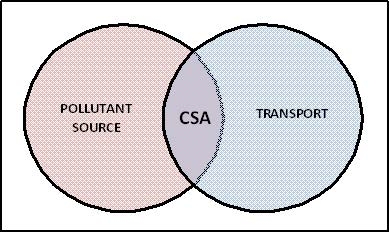
The concept of critical source areas (CSA).
Approaches to Identifying Critical Source Areas
NIFA-CEAP Approaches. Most of the land treatment in the NIFACEAP projects had already been implemented under previous voluntary programs and not deliberately targeted to CSAs. Three projects involved retrospective analyses to assess the degree to which conservation practices had been implemented on CSAs.
The Goodwater Creek Watershed (MO) NIFA-CEAP project used two modeling approaches to identify CSAs. O’Donnell et al. (2011) used outputs from a calibrated Soil and Water Assessment Tool (SWAT) model to identify critical fields for sediment and atrazine losses in the watershed. The modeling exercise simulated use of filter strips and other conservation practices and found adoption of these practices would be necessary on 19% and 29% of the most critical fields in the watershed to reduce atrazine and NO3-N loads, respectively. In addition, project researchers used a calibrated Agricultural Policy/Environmental eXtender (APEX) model to identify critical management areas within a 35- hectare field based on runoff, sediment, and dissolved atrazine contributions (Mudgal et al. 2011). Simulation results confirmed that areas with a shallow claypan were more prone to generate high runoff and both atrazine and sediment loads.
Subsequently, two simple spreadsheet- based tools were developed to identify CSAs for runoff and atrazine using readily available data (slope, hydraulic conductivity, and depth to claypan) (Mudgal et al. 2011). Unfortunately, most of the conservation practices applied in the watershed from 1993 to 2003 had been implemented on noncritical areas.
In the Little Bear River Watershed (UT) NIFA-CEAP project, de la Hoz et al. (2008) conducted a geographic analysis of critical sediment sources in the watershed using a series of overlays based on the Universal Soil Loss Equation (USLE). The overlays included information on soil, slope, land use, and proximity to a water course and indicated about 13% of the watershed area was in the highest nonpoint source risk category. About 26% of these identified critical areas had received some previous land treatment, suggesting that a degree of targeting had occurred during the USDA Hydrologic Unit Area project. However, 75% of conservation practices had been applied to fields with low potential pollutant loads.
In the Cheney Lake Watershed (KS) NIFA-CEAP project, Nelson et al. (2011) used a geographical information system based on the Revised Universal Soil Loss Equation (RUSLE, version 2) to better identify CSAs based on erosion losses. Fields were divided into those with greater (top 20% of the watershed) and lesser erosion rates. The CSAs within the watershed were those landscape positions with the highest erosion rates. These areas deliver an estimated 56% of the total sediment load. Little difference could be detected in rates of conservation practice implementation for CSA fields and other fields. Only 22% of implemented conservation practices were located in the CSAs. Fields with Conservation Reserve Program grasslands were often found in these priority areas because this practice was targeted to highly eroding land in the watershed. The converse was true of conservation tillage, which was not used as frequently in the CSAs.
Other Approaches. Past approaches to identifying CSAs have ranged from simple inventories to complex models as our technology and approaches have continued to evolve.
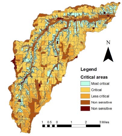
Critical area determination in Goodwater Creek watershed (MO)
(Baffaut and Mudgal, personal communication).
Miscellaneous Approaches
- The likely areas contributing high P s in the Lake Champlain Basin were identified by their hydrologic unit codes (HUCs) using simple export coefficients and loading functions (Meals and Budd 1998).
- A soil moisture model was combined with land use, soil phosphorus status, and nitrogen balance information to predict CSAs from agricultural land (Pionke et al. 2000).
- A simplified Universal Soil Loss Equation (USLE) factor map was used to delineate high-risk areas for phosphorus and sediment export (Sivertun and Prange 2003).
- Critical source areas were identified by overlaying P application rates and times, soil test P, distance to waterways, and runoff risk; catchment rankings were found to be positively correlated with measured in-stream P concentrations (Hughes et al. 2005).
- Individual fields were ranked for P loss risk through surface runoff based on internal and external drainage characteristics mapped with a highresolution digital elevation model (DEM) (Sonneveld et al. 2006).
Topographic Index Approaches
Many researchers have applied the concept of the topographic index to CSA identification. A topographic index is an estimate of the potential for soil saturation— and therefore generation of surface runoff —of a land area based on slope and catchment area (Bevin and Kirkby 1979).
- A topographic index was added to weight export coefficients by landscape position to map spatially distributed gradients of pollutant-loading risk (Endreny and Wood 2003).
- A high-resolution mapping and topographic index analysis was combined with field information to assess nutrient loss risk on a field-by-field basis in an agricultural catchment (Heathwaite et al. 2005).
- Five approaches to CSA delineation, including curve number, Phosphorus Index, drainage density, topographic index, and topographic index plus impervious cover were compared; using a topographic index gave the best results (Srinivasan and McDowell 2007, 2009).
- Others have modified the USDA Soil Conservation Service curve number equation for variable source area hydrology and incorporated it into the Generalized Watershed Loading Function (GWLF) model (Haith and Shoemaker 1987) to spatially distribute the runoff response according to a topographic index (Schneiderman et al. 2007, Easton et al. 2008, Rao et al. 2009).
- A topographic index was coupled with a spatially explicit mass-balance model to simulate the development of P source hot spots over time in a Vermont watershed (Meals et al. 2008a, 2008b).
- A GIS approach was used with a modified topographic index based on variable source area hydrology to target CSAs for conservation buffer placement in New Jersey. The topographic index was found to reasonably predict runoff generation in the watershed. The GIS-targeted conservation buffer scenarios appear to be more cost-effective than the conventional riparian buffer scenarios (Qiu 2009).
- A topographic index, SWAT, and proximity to surface water were used to identify CSAs for P in an agricultural river basin in northwest Vermont (Winchell et al. 2011). Land in a corn-hay rotation produced the greatest contribution (29%) of the total watershed P load from upland sources. The SWAT model was able to evaluate and rank the P loads associated with specific landscape units—from major subwatersheds, through smaller subbasins, down to the highest resolution landscape areas.
Targeting Critical Source Areas
Watershed management strategies to reduce nonpoint source pollutant export could be more cost-effective and watershed conservation projects more successful if conservation practices were targeted to CSAs (Sharpley 1995, Pionke et al. 2000, Yang and Weersink 2004, Gburek et al. 2000). Walter et al. (2001) proposed that a 25% reduction in watershed soluble P loading from New York agricultural watersheds was possible by adjusting the timing and location of manure application only on hydrologically sensitive areas. Winchell et al. (2011) reported that modeled P load reductions from implementing selected conservation practices targeted to the highest priority CSAs were two to three times greater than those achieved by traditional completely voluntary implementation of the same practices at the same level.
Because of the importance of CSAs, it is essential that these landscapes be identified. Identifying the pollutant of concern and its source and understanding hydrology are the first steps to critical area identification. Sometimes identifying the critical area will be straightforward, such as a water-quality problem due to N and fields with drainage tiles; the critical area becomes drained fields. Critical source areas for sediment losses from stream banks may require walking the streams to find the impacted areas. Erosion or P losses from uplands may be more complex and will require one of the methods described. To use financial resources effectively and to protect water quality, CSAs should be identified before any conservation practices are implemented.
References
Bevin, K. J. and M. J. Kirkby. 1979. A physically based variable contributing area model of basin hydrology. Hydrol. Sci. Bull. 24(1):43-69. ↲
de la Hoz, E. A., D. Jackson- Smith, and J. Horsburgh. 2008. Assessing the spatial distribution of agricultural conservation practices implemented along a Northern Utah watershed: Did practices target critical areas? Little Bear CEAP. Logan, UT: Utah State University Cooperative Extension. ↲
Dunne, T. and R. D. Black. 1970. Partial area contributions to storm runoff in a small New England watershed. Water Resour. Res. 6:1296-1311. ↲
Easton, Z. M., M. T. Walter, and T. S. Steenhuis. 2008. Combined monitoring and modeling indicate the most effective agricultural best management practices. J. Environ. Qual. 37:1798– 1809. ↲
Endreny, T. A. and E. F. Wood. 2003. Watershed weighting of export coefficients to map critical phosphorus areas. J. Am. Water Resour. Assoc. 39(1):165- 181. ↲
Frankenberger, J. R., E. S. Brooks, M. T. Walter, M. F. Walter, and T. S. Steenhuis. 1999. A GIS-based variable source area hydrologic model. Hydrol. Process. 13:805-822. ↲
Gburek W. J., A. N. Sharpley, and D. B. Beegle. 2007. Incorporation of variable-source-area hydrology in the Phosphorus Index: A paradigm for improving relevancy of watershed research. In D. L. Fowler (ed.), Proceedings, Second Interagency Conference on Research in the Watersheds, May 2006 (pp. 151-160). Otto, NC: Coweeta Hydrologic Laboratory, USDA Forest Service, Southern Research Station. ↲
Gburek, W. J., A. N. Sharpley, and G. J. Folmar, 2000. Critical areas of phosphorus export from agricultural watersheds. In A. N. Sharpley (ed.), Agriculture and Phosphorus Management (pp. 83- 104). Boca Raton, FL: Lewis Publishers. ↲
Haith, D. A. and L. L. Shoemaker. 1987. Generalized watershed loading functions for stream flow nutrients. Water Resour. Bull. 23(3):471-478. ↲
Heathwaite, A. L., P. F. Quinn, and C. J. M. Hewett. 2005. Modelling and managing critical source areas of diffuse pollution from agricultural land using flow connectivity simulation. J. Hydrol. 304:446–461. ↲
Heathwaite, A. L., A. N. Sharpley, and W. J. Gburek. 2000. Integrating phosphorus and nitrogen management at catchment scales. J. Environ. Qual. 29:158-166. ↲
Hughes, K. J., W. L. Magette, and I. Kurz. 2005. Identifying critical source areas for phosphorus loss in Ireland using field and catchment scale ranking schemes. J. Hydrol. 304:430–445. ↲
Meals, D.W. and L. F. Budd. 1998. Lake Champlain Basin nonpoint source phosphorus assessment. J. Am. Water Resour. Assoc. 34(2):251–265. ↲
Meals, D. W., E. A. Cassell, D. Hughell, L. Wood, W. E. Jokela, and R. Parsons. 2008a. Dynamic spatially explicit mass-balance modeling for targeted watershed phosphorus management, I. Model development. Agriculture, Ecosystems and Environment 127:189-200. ↲
Meals, D. W., E. A. Cassell, D. Hughell, L. Wood, W. E. Jokela, and R. Parsons. 2008b. Dynamic spatially explicit mass-balance modeling for targeted watershed phosphorus mass-balance modeling for targeted watershed phosphorus management, II. Model application. Agriculture, Ecosystems and Environment 127:223-233. ↲
Mudgal, A., C. Baffaut, S.H. Anderson, E.J. Sadler, N.R. Kitchen, K.A. Sudduth, and R.N. Lerch. 2012. Using the Agricultural Policy/Environmental eXtender to develop and validate physically based indices for the delineation of critical management areas. Journal of Soil and Water Conservation 67(4):282- 297. ↲
Nelson, N., A. Bontrager, K. Douglas-Mankin, D. Devlin, P. Barnes, and L. Frees. 2011. Cheney Lake Watershed: Prioritization of Conservation Practice Implementation. Kansas State University Agricultural Experiment Station and Cooperative Extension Service, Publication MF3031. Manhattan, KS. ↲
O’Donnell, T. K., K. W. Goyne, R. J. Miles, C. Baffaut, S. H. Anderson, and K. A. Sudduth. 2011. Determination of representative elementary areas for soil redoximorphic features identified by digital image processing. Geoderma 161(3-4):138-146. ↲
Osmond, D., D. Meals, D. Hoag, and M. Arabi (eds). 2012. How to Build Better Agricultural Conservation Programs to Protect Water Quality: The National Institute of Food and Agriculture Conservation Effects Assessment Project Experience. Ankeny, IA: Soil and Water Conservation Society. ↲
Pionke, H. B., W. J. Gburek, and A. N. Sharpley. 2000. Critical source area controls on water quality in an agricultural watershed located in the Chesapeake Basin. Ecol. Eng. 14: 325–335. ↲
Qiu, Z. 2009. Assessing critical source areas in watersheds for conservation buffer planning and riparian restoration. Environ. Manage. 44(5):968-980. ↲
Rao, N. S., Z. M. Easton, E. M. Schneiderman, M. S. Zion, D. R. Lee, and T. S. Steenhuis. 2009. Modeling watershed-scale effectiveness of agricultural best management practices to reduce phosphorus loading. J. Environ. Manage. 90:1385-1395. ↲
Schneiderman, E. M., T. S. Steenhuis, D. J. Thongs, Z. M. Easton, M. S. Zion, A. L. Neal, G. F. Mendoza, and M. T. Walter. 2007. Incorporating variable source area hydrology into a curve-number-based watershed model. Hydrol. Process. 21:3420– 3430. ↲
Schoumans, O. F. and A. Breeuwsma. 1997. The relation between accumulation and leaching of phosphorus: Laboratory, field and modelling results. In H. Tunney, O. T. Carton, P. C. Brookes, and A. E. Johnston (eds.), Phosphorus Loss from Soil to Water (pp. 361-363). Cambridge, England: CAB International Press. ↲
Sharpley, A. N. 1995. Dependence of runoff phosphorus on extractable soil phosphorus. J. Environ. Qual. 24:920–926. ↲
Sivertun, A. and L. Prange. 2003. Nonpoint source critical area analysis in the Gisselo watershed using GIS. Environ. Modelling Software 18:887-898. ↲
Sonneveld M. P. W., J. M. Schoorl, and A. Veldkamp. 2006. Mapping hydrological pathways of phosphorus transfer in apparently homogeneous landscapes using a high-resolution DEM. Geoderma 133:32-42. ↲
Srinivasan, M. S. and R.W. McDowell. 2007. Hydrological approaches to the delineation of critical-source areas of runoff. New Zealand J. Agri. Res. 50:249-265. ↲
Srinivasan M. S. and R. W. McDowell. 2009. Identifying critical source areas for water quality: 1. Mapping and validating transport areas in three headwater catchments in Otago, New Zealand. J. Hydrol. 379: 54- 67. ↲
Walter, M. T., Brooks, E. S., Walter, M. F., Steenhuis, T. S., Scott, C. A., Boll, J. 2001. Evaluation of soluble phosphorus loading from manure-applied fields under various spreading strategies. J. Soil Water Cons. 56(4):329-335. ↲
Ward, R. C., 1984. On the response to precipitation of headwater streams in humid areas. J. Hydrol. 74:171-189. ↲
White, M. J., D. E. Storm, P. R. Busteed, S. H. Stoodley, S. J. Phillips. 2009. Evaluating nonpoint source critical source area contributions at the watershed scale. J. Environ. Qual 38: 1654-1663. ↲
Winchell, M., D. W. Meals, S. Folle, J. Moore, D. Braun, C. DeLeo, K. Budreski, and R. Schiff. 2011. Identification of Critical Source Areas of Phosphorus within the Vermont Sector of the Missisquoi Bay Basin. Final Report to The Lake Champlain Basin Program. Montpelier, VT: Stone Environmental, Inc. ↲
Yang, W. and A. Weersink. 2004. Cost-effective targeting of riparian buffers. Can. J. Agric. Econ. 52:17-34. ↲
Related Resources
Line, D.L. and J. Spooner. 1995. Critical Areas in Agricultural Nonpoint Source Pollution Control Projects: The Rural Clean Water Program Experience. NCSU Water Quality Group, Raleigh, NC.
Prepared by
Donald W. Meals, Ice. Nine Environmental Consulting
Andrew N. Sharpley, University of Arkansas
Deanna L. Osmond, North Carolina State University
Information
For more information about the NIFA-CEAP Synthesis, contact Deanna Osmond, NC State University.
Lessons Learned from the NIFA-CEAP
Acknowledgments
The authors are grateful for the funding supplied by the USDA National Institute of Food and Agriculture (NIFA) and Natural Resources Conservation Service (NRCS) (Agreement No. 2007- 51130-18575). We want to thank all NIFA-CEAP project personnel for their help with this publication, our site visits, and our information-gathering efforts. In addition, we greatly appreciate all the time spent by key informants during our interviews with them. We also wish to thank the USDA CEAP Steering Committee and USDA NIFA Committee for Shared Leadership for Water Quality for their comments, questions, and advice during this synthesis project, as well as a special thanks to Lisa Duriancik of NRCS.
This material is based upon work supported in part by the National Institute of Food and Agriculture and the Natural Resources Conservation Service, U.S. Department of Agriculture, under Agreement No. 2007-51130- 18575. Any opinions, findings, conclusions, or recommendations expressed in this publication are those of the author(s) and do not necessarily reflect the view of the U.S. Department of Agriculture. USDA is an equal opportunity provider and employer.
Citation
Meals, D. W., A. N. Sharpley, and D. L. Osmond. 2012. Lessons Learned from the NIFA-CEAP: Identifying Critical Source Areas. NC State University, Raleigh, NC.
Publication date: Jan. 1, 2012
Revised: Dec. 18, 2023
N.C. Cooperative Extension prohibits discrimination and harassment regardless of age, color, disability, family and marital status, gender identity, national origin, political beliefs, race, religion, sex (including pregnancy), sexual orientation and veteran status.