Every new design is an experiment into new territory. Enlarging what is possible and taking calculated but educated risks with your client’s money and your reputation are the spirits of engineering. To be successful, engineering design relies on knowledge and judgment. There is no easy way to calculate the accurate cooling times and refrigeration loads for any combination of fans, produce, and containers. Despite the availability of numerous heat transfer equations, the best results may be just estimates. There are published data on various cooling equipment/produce combinations, but the likelihood of finding the exact data fit is slim. Nevertheless, having a good understanding of heat transfer is essential in leveraging the available published data for use in your particular application.

Whenever you design and build a new facility, it is essential that you collect operational data for your current reference and use in later designs. In fact, post construction testing is frequently a requirement of a construction contract. This requires experimental design and instrumentation to test empirically what has been built and how to improve the operation. Most engineers understand the importance of data collection for publishing as a service to others and for maintaining their own references.

Collecting data may be the simple part. Today, readily available automated data collection systems make it possible to collect millions of data points in a very short period. The challenge is interpreting the data. Engineers need to know how to use different statistical techniques and how to interpret the results, which may not match what they expected.

There are many acceptable electronic thermometers, hygrometers, and airflow meters available for researching and recording postharvest cooling and storage data. It is essential that you use only high quality instruments. Over time and in the conditions encountered in coolers, these instruments tend to lose their calibration. Since this is a particular problem with electronic humidity sensors, even the most expensive sensors require testing and calibration on an annual basis. For this evaluation, a simple sling hygrometer, as shown in Figure PS-1, is the gold standard. This includes two identical thermometers, a dry bulb thermometer and a wet bulb thermometer. The bulb of the wet thermometer has its bulb surrounded by a wet cotton “sock,” which is actually a piece of shoestring. When this is whirled through the air, the dry bulb records the air temperature and the wet bulb is cooled by evaporation. The lower the humidity, the greater the cooling. The actual relative humidity is identified when the two temperatures are compared to a scale.

Room temperature is best measured by a good quality thermometer that is controlled by a thermostat or programmable logic controller (PLC) sensing with a resistance temperature detector (RTD). It makes no sense to build a million-dollar postharvest facility, fill it with produce worth several hundred thousand dollars, and then monitor and control the facility with the least expensive temperature sensor. Even good thermostats must be calibrated at the beginning of each cooling season to assure that they agree within one or two degrees with a calibrated thermometer. The thermometer and the sensing element of the thermostat must be positioned near each other in a location where they may be easily seen, and if possible, where they are away from the direct airflow from the refrigeration coils, the exterior walls or doors, and vents. The temperature and humidity sensors should always be positioned at the place that is being monitored. For example, if you are interested in knowing the temperature in the center of a pallet bin of produce, it is best to put the sensing element in the center of the bin, and not on the wall by the door.

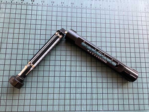
Figure PS-1. A sling hygrometer (psychrometer) exposes a dry bulb and a wet bulb thermometer to moving air. Relative humidity can be found by comparing the difference between the temperatures.

Source: M. Boyette.

×

Figure PS-1. A sling hygrometer (psychrometer) exposes a dry bulb and a wet bulb thermometer to moving air. Relative humidity can be found by comparing the difference between the temperatures.

Source: M. Boyette.

Print Image

In one example, you have designed a forced-air cooling facility that is operated primarily to cool produce in pallet bins before their transport to a processing facility. You were assigned to select the fans for the six cooling lanes. Each cooling lane is 60 ft long with floor space for 24 pallets (12 in. two parallel rows). Although you think the fans you have selected have sufficient capacity, there are some questions about the inevitable air leakage between the pallets and the density of the produce. According to your calculations and expert judgment, you predicted that this arrangement would yield a ⅞ cooling time of about 3½ hours. The facility owner is a bit skeptical about your decision.

Today at the location, workers are bringing jalapeno peppers in 1000-lb bulk pallet bins directly from the field. The peppers have been picked at different times during the day and from different locations, which means that the peppers are not all the same temperature. You discover that the peppers picked early in the morning are as much as 18F° degrees cooler than those picked at mid-day. As the bins are being unloaded and positioned in the cooler, you place six blue-tooth enabled temperature sensors to monitor the progress of the cooling.

The correct location to position sensors is important and should never be a matter of convenience. Sensors are the eyes and ears of the cooling facility and must be located at the best vantage points for gathering the most information, which are located among the produce. In a forced-air cooling environment, the best location for the sensors is on the downstream side of the bins inside the plenum and inside, or at least in contact, with an individual piece of produce that in this case is a single jalapeno pepper. This should provide the truest measure of the produce temperature.

With cracks between pallets and boxes, there may be some air that penetrates the produce containers. If the air flow rate, Q, is different from one end of the cooling lane to the other, two sensors can be placed near the fan, two in the middle rows, and two at the end opposite the fan.

Before the introduction of inexpensive electronic data collection modules as shown in Figure PS-2, collection of cooling data was long, tedious, and often cold. Modern data collection modules, which can be programmed to collect time-stamped data at various intervals, are able to operate unattended for days, weeks, or months when necessary. However, data collection at very short intervals is not encouraged because the result can be very large, unwieldy data sets. For most postharvest cooling tests, intervals of no less than 5 or 10 minutes are acceptable.

In the example with jalapeno peppers, the sensors have been programmed to sample the temperature every 10 minutes and transmit the data, via Bluetooth, to the telephone. The room temperature is kept at a constant 45°F. After several hours, the data can be downloaded into an Excel file as shown in Table PS-1.

Source: M. Boyette

The data show that there was an 18F° initial difference between the pallet #2 sensor and the pallet #3 sensor. It appears that the temperature for all pallets after 3½ hours was below 50°F and that all temperatures were within 2 F° of each other. This indicated active cooling throughout the bins.

There are now two related questions to answer from the cooling data:

1. Despite the fact that the peppers had a range of temperatures, did all the peppers cool in the predicted ⅞ cooling time of 3½ hours? The forced-air cooling rate is very dependent on the convection coefficient, h, and with forced convection, is influenced within limits by the airflow rate. Are the fans too small, too big, or just right?
2. If not, why not? Were all the bins of peppers slow to cool because the fan was undersized or because the airflow was uneven between bins because of leakage between bins and/or uneven negative pressure distribution?

By converting a data table to a graph, the data will often reveal trends and relationships that are impossible to see by looking only at the numbers. Figure PS-3 below is Table PS-1 that has been converted to a graph.

The graph shows that the bins that were warmer at the beginning initially cooled faster than those that were cooler. This makes sense given that the rate of heat transfer is driven by Δ T. The greater the Δ T, the faster the cooling. As the bins cooled, the differences in temperature grew less but were still proportional to the initial temperatures. All curves converged to the room temperature of 45°F. This cooling curve assumes the form of y= e^−xt where “x” is the system characteristic. The value of x is influenced by characteristics of a particular cooling situation such as the size and shape of the produce, the rate of heat transfer through the interior of the produce, the heat transfer from the surface of the produce, and the velocity of the cooling air. The velocity of the cooling air is influenced by the size and types of fans and also by the presence, size, shape, and orientation of the ventilation openings in the packaging. The variable x is not influenced by the starting pulp temperature of the produce or the room temperature as long as the room temperature remains constant. For this reason, determining the value of x is an excellent way to compare the effects of different packaging, airflow rates, and product sizes on the cooling rate without being concerned with the actual produce and air temperatures.

Since the proportionality of differences appears to be maintained throughout the time of cooling, it is likely that the system characteristics (x) are the same or similar at all six of the test bins. Assuming that the size of the peppers in all bins are similar in size and/or size distribution, it is also likely that the airflow rate is uniform and the negative pressure distribution is uniform throughout the plenum space between the rows of bins. This is a good result, although questions remain about the ⅞ cooling times.

This is where a normalized temperature is important. Normalization is the process of reducing measurements to a neutral or standard scale so that different measurements may be easily compared. Here again is Newton's law of cooling equation: y= e^−xt

This class of mathematical equations, known as inverse exponentials, are functions that decrease at an ever decreasing rate. In the example about produce cooling, the temperature is decreasing with time, but the rate of decrease (expressed as degrees per minute) is also decreasing and slowing. The reason is simple. The difference in temperature, Δ T, is the driving force of heat transfer. As the magnitude of Δ T decreases, the rate of heat transfer decreases. This is exactly what happens to the flow of water from a bucket with a hole in the bottom. When the bucket is full, the water flows rapidly, but as the level of water drops, the rate of flow decreases. This happens because the rate of flow is driven by the head of water.

In Equation 1, above, the variable y is the normalized (or dimensionless) temperature that ranges between 0 and 1 (0 < y < 1). At any given moment in the cooling cycle, y may be determined by equation:

y = [(T_t −T_e) / (T_s− T _e)]

Where:

T_t = the temperature at any time, t

T_e = the room (end) temperature, 45°F in the example

T_s = the starting temperature (that varies with bins)

If we rearrange terms and set y = 0.125 (the normalized temperature is 0.125 after the produce has cooled ⅞ (.875) of the way from the starting temperature to the room temperature), we have the following:

T_t = y(T_s−T_e) + T_e

The starting temperatures for the six sensors are:

#1: 86°F, #2: 96°F, #3: 78°F, #4: 82°F, #5: 93°F, #6: 89°F

Substituting:

#1: T_t = (.125) (86−45) + 45 = 50.1°F

#2: T_t = (.125) (96−45) + 45 = 51.3°F

#3: T_t = (.125) (78−45) + 45 = 49.1°F

#4: T_t = (.125) (82−45) + 45 = 49.6°F

#5: T_t = (.125) (93−45) + 45 = 51.0°F

#6: T_t = (.125) (89−45) + 45 = 50.5°F

Table PS-1 shows that all ⅞ cooling times were reached at the 3-hour mark, a half-hour before the target of 3½ hours. Thus, the data analysis reveals that the fans were sized adequately, a conclusion that would please the no longer skeptical owner and ensure your continuing employment.

Knowing the actual numerical value of x for a particular cooling situation is very useful for comparing different situations. For example, determining the value of x is an excellent way to compare the effects of different types of packaging, airflow rates, and product sizes on the cooling rate without being concerned with the actual produce and air temperatures.

Calculating the value of x in the example is very simple. If we solve Newton’s equation for x and substitute actual data, we can obtain x. For example, at about 180 minutes, the sensors have all reached their ⅞ temperature and substituting: y = e^−xt

Then taking the natural log of both sides, Ln(y) = −xt

x = −(Ln(y) / t = −[Ln(.125) / 180] = −0.0116

For your convenience, the values of x have been calculated and tabulated for ⅞ cooling times from 5 to 300 minutes in Table PS-2.

Figure PS-2. Bluetooth-enabled programmable multichannel data collection module.

Source: M. Boyette.

×

Figure PS-2. Bluetooth-enabled programmable multichannel data collection module.

Source: M. Boyette.

Print Image

Figure PS-3. Graph of the data in Table PS-1.

Source: M. Boyette.

×

Figure PS-3. Graph of the data in Table PS-1.

Source: M. Boyette.

Print Image

Despite the great utility of Newton's law of cooling equations, y= e^−xt, the law is an ideal that will generate reasonable answers. If you opt to use some data and not others, you should be sure your actions are justified by established facts. It is not ethical to “cherry pick” data to support pre-conceived results.

However, there might be a good reason not to include some portion of cooling data you have collected from your analysis. Figure PS-4 shows data collected from a strawberry cooling experiment. The lowest dashed line is the room ambient temperature and the line above is the ⅞ temperature of the last strawberries to cool. The other curves represent data from temperature sensors embedded inside individual strawberries positioned at various places. Cooling required some time to stabilize. For the first 10 minutes, some strawberries were cooling at different rates and some remained the same, which was far from the ideal of Newton’s Law. Applying Newton’s Law makes no sense for the initial portion of this particular test.

The factors that influence the cooling rate (airflow, produce shape and size, and packaging) do not change from the beginning of the test to the end with the exception of the ambient room temperature of each position. (Not shown is the actual ambient room temperature. The room set point is 35°F.) Since we have just placed a heat load into that stream, it is not surprising to see the air temperature rise and then fall later. As the test proceeds, the ambient room temperature becomes more stable as it approaches its set point, and the requirement of Newton’s Law for the ambient temperature to be constant is then satisfied.

Since the factors that influence the cooling time are constant, the “x” or system coefficient should remain the same and the shape of the curve at any point should be the same. Ideally, after the initial period of stabilization, any point along the line should yield the same solution to the equation, y = e^−xt. Thus, it is acceptable to select cooling data from the middle third of the cooling test as representative.

Figure PS-4. Graph of the data from a strawberry cooling test.

Source: M. Boyette.

×

Figure PS-4. Graph of the data from a strawberry cooling test.

Source: M. Boyette.

Print Image