
Introduction
Soil sampling is the first step in generating field-specific information to make lime and fertilizer decisions. Selecting an appropriate sampling strategy ensures that the soil in a field is collected in a manner that produces the most accurate and reliable soil test results. Because soils in agricultural fields can vary significantly, use a sampling strategy that best captures that variation. Proper sampling is particularly important when a site-specific management approach is embraced.
In site-specific management, the management of the crop and underlying soil occurs at a scale smaller than that of the whole field. Under this management approach, separate soil samples are collected from areas that are smaller than the generally recognizable subunits within a field. Soil amendments such as fertilizer and lime are then applied at rates based on soil test results and plant needs specific to that area, thus optimizing the overall production in the field. Site-specific management results in a variable rate of applied amendments. The required amount of amendments to a field varies based on the soil nutrient status (soil tests) and crop grown, but is also influenced by factors such as soil texture, drainage, and landscape position.
Modern technologies including GPS (Global Positioning System), GIS (Geographic Information Systems), FMIS (Farm Management Information Systems), and Variable Rate Technology (VRT) allow producers to manage soils and amendments with greater precision. Site-specific soil sampling provides the foundation for many lime and fertilizer decisions enabled by these technologies. Site-specific soil sampling is the basis for
- identifying the spatial distribution of nutrient deficiency and sufficiency within fields;
- increasing lime and fertilizer use efficiency by variably distributing lime, nutrients, and other amendments based on the spatial distribution of soil properties and crop requirements;
- minimizing potential for nutrient loss from fields by overapplication; and
- optimizing production through the targeted use of agricultural amendments.
To best utilize site-specific soil sampling, you need a clear understanding of the benefits and limitations of each sampling strategy, as well as knowledge surrounding the tools and process used to develop the sampling plans. This publication provides information to help select and develop soil sampling strategies used in the site-specific management of agricultural fields.
Site-Specific Soil Sampling Terms
Base map: A background map used within a GIS that enables the digitization of spatially accurate field boundaries. Typically, the base map is an aerial photograph referenced to locations on Earth’s surface (georeferenced). Field boundaries are created by tracing the border of a field as it is visually identified in the base map.
Cell sampling: A sampling approach in which a field is divided into a grid of uniformly sized cells, and each cell is sampled independently. A single composite sample is collected throughout each cell and used to characterize soil properties within a cell.
Composite soil sample (single versus multiple): A single composite sample contains 15 to 20 soil cores collected at random locations throughout a field or area. In comparison, multiple composite samples involve collecting soil samples (15 to 20 cores per sample) at multiple locations within a field, as determined by the site-specific sampling approach (for example, point, cell, or zone).
Differential correction: A GPS technique that uses an additional signal to enhance the accuracy of a position collected using a GPS receiver. Different sources of differential correction exist and vary in cost and in their ability to correct for the normal errors in a GPS-determined position.
FMIS (Farm Management Information System): Software designed to support various aspects of an agricultural operation. Unlike a GIS, the software helps organize and manage farm activities such as record-keeping, work scheduling, purchasing, data collection and storage, and map making. The levels of support and functionality differ based on the software and intended use.
GIS (Geographic Information System): Software used to visualize, analyze, and describe patterns and relationships between layers of spatial data. GIS is the foundation for most Farm Management Information Systems.
GPS (Global Positioning System): A global navigation and positioning system that uses satellites to locate positions on Earth’s surface. A GPS receiver uses signals broadcast from satellites to determine its position (for example, latitude, longitude, and elevation). A GPS receiver can either record, or navigate to, different locations within a field to collect a site-specific soil sample.
Grid: A network of lines superimposed on a field map to assist in partitioning the field into smaller areas. The resulting cells are the areas sampled in a grid cell sampling approach, while the intersecting lines (or the centers of the resulting cells) indicate the location of samples in a point sampling approach.
Interpolation: A mathematical technique that uses neighboring points with known values to estimate values at unsampled locations. In a point sampling approach, interpolation is used to create a spatially continuous model of a soil property or recommended value. Common interpolation techniques include Inverse Distance Weighted (IDW), Spline, and Kriging.
Point sampling: A sampling approach in which soil samples are collected from relatively small, localized areas (points) systematically located throughout the field. A uniform grid placed over the field boundary typically guides the design of the sampling plan. After point sampling, interpolation is used to estimate the soil properties at unsampled locations. Interpolation creates a continuous representation of the measured soil property that is then used to develop a prescription rate map across the entire field.
Prescription rate map: A digital map used in variable rate technology to control the rate (or amount) of amendment (for example, lime, fertilizer, or water) to apply based on the location in the field.
Shapefile: The data format used by most GIS/FMIS software to store spatial data (for example, field boundaries, point locations, or the polygons that represent grid cells). A shapefile is stored as a collection of files with a common name but different file extensions (for example, .shp, .shx, and .dbf).
Variable rate controller: The field computer and software mounted inside a tractor that control the rate of application based on location. Most rate controllers work by altering the output or flow of applicator pumps or by controlling regulating valves.
VRT (Variable Rate Technology): A technology that enables the variable application of inputs (for example, fertilizer, lime, or water) by location. The basic components are a field computer, a variable rate controller, a GPS receiver, and a prescription rate map indicating where and how much material to apply.
WASS (Wide Area Augmentation System): A satellite-based source of differential correction used to enhance the accuracy of a GPS receiver. Developed for the Federal Aviation Administration (FAA), the signal is free and available anywhere in the United States. Most GPS receivers use this signal to achieve a horizontal accuracy of 10 to 15 feet (3 to 5 meters).
Zone sampling: A site-specific sampling scheme that is designed to split a field into zones containing similar soil or crop characteristics. Zones are managed as separate areas within the field and are often based on areas that exhibit similar field variability due to inherent soil properties (for example, soil texture and drainage), management history (for example, drainage, land shaping, spreader patterns, and previous land use), or historic production levels. This approach reduces the number of samples required while still recognizing zones of differing nutrient status and fertility requirements. Zone sampling typically defines smaller, more detailed areas compared to those defined under standard sampling guidelines. Multiple spatial data layers are typically combined (for example, historic yield and soil type) to develop zones.
How to Collect Georeferenced Soil Samples
1. Delineate field boundaries.
Field boundaries are best delineated by using either a portable GPS receiver or by tracing boundaries from an aerial image used as a base map. For this purpose, the GPS manufacturer specifications should indicate horizontal accuracies of about 3 meters or better. Most GPS receivers with this level of accuracy cost less than $500 and use a free differential correction service known as WASS. If greater accuracy is desired, you may buy or rent GPS receivers designated as mapping-grade or survey-grade. Mapping-grade receivers are typically accurate to 1.5 to 7 feet (0.5 to 2 meters) and cost about $2,000, while survey-grade receivers can pinpoint locations to within a few inches but typically cost more than $10,000. Survey-grade receivers require an additional differential correction signal provided either from a local base station or from a paid subscription service. For a one-time $500 subscription fee, the North Carolina Geodetic Survey will provide the real-time differential corrections required to achieve the highest accuracy with a survey-grade GPS receiver.
To map field boundaries using a GPS, either walk or drive along the field’s edge and record the GPS positions. Rectangular fields are best delineated using GPS locations at field corners, while irregularly shaped fields necessitate the GPS to log points continuously along the field boundary. After data collection, the files are downloaded from the GPS receiver and loaded into a GIS or FMIS to guide the development of the base map. Data formats used by GIS or FMIS can vary, but both types of software should accept a shapefile as the input format.
An alternative to developing field boundaries with a GPS is to trace the outline of your fields using GIS/FMIS software and an aerial photograph or photographs as a base map. The National Agriculture Imagery Program (NAIP) acquires aerial imagery yearly during the agricultural growing season. You may download the images free via the U.S. Department of Agriculture’s Farm Service Agency website. The typical process used to develop field boundaries without a GPS involves locating and downloading the aerial photographs for your field locations, loading the aerial photographs into a GIS/FMIS, creating an empty shapefile to store and save the field boundaries, and tracing each field boundary using the drawing tools in the software and the aerial photographs as a visual reference. Compared to GIS, most FMIS software makes the creation of field boundaries simpler by providing georeferenced imagery as base maps and a simplified set of tools designed for creating field boundaries.
2. Select a sampling strategy: grid cell, point, or zone sampling.
Site-specific soil sampling strategies include cell (Figure 1), point (Figure 2), and zone (Figure 3) methods as well as combinations of each called “hybrid” approaches (Figure 8).
Cell sampling is a sampling technique in which a field is subdivided into uniformly sized squares (or rectangles) called cells. The cells are created by placing a grid over the field boundary (base map). Soil samples are collected within each cell using a traditional composite sample approach; cores are collected from locations within each cell and mixed to generate a single composite sample (Figure 4). The resulting soil analyses represent average soil characteristics within each cell. The soil test data are then used to develop amendment recommendations for each cell.
Each cell within the grid is typically 1 to 3 acres for most fields in North Carolina. A smaller cell size is justified with higher value crops or if greater soil variability is expected. Selecting a cell size is a practical decision based on the added costs of collecting more samples compared to the potential benefits of site-specific management.
To use the cell sampling approach, collect 15 to 20 cores from random locations within each cell (Figure 4a). Soil samples may be collected via a staggered pattern that facilitates forward walking or vehicle movement to the next cell (Figure 4b). To avoid spatial bias, avoid collecting cores in smaller clusters (Figure 4c) or in a straight line (Figure 4d). A sample that contains cores from only a small, localized area within the cell can result in a misrepresentation of the underlying soil properties and an inaccurate recommendation. Samples collected along straight lines may unintentionally correspond to previously banded fertilizer applications, vehicle traffic, or localized removal of nutrients along rows.
Point sampling is typically recommended when little information is known about the underlying field-scale variability. As with cell sampling, a uniform 1- to 3-acre grid is placed over the field boundary, and soil samples are collected at point locations on the grid (Figure 5). The grid is used to identify sample locations at the intersection of the grid lines (Figure 5a and Figure 5d), every other grid intersection (Figure 5b), or random spots within each grid cell (Figure 5c). Once the plan is developed, the sample locations are loaded into a GPS and used to navigate to the points. At each point, a composite sample is collected. To collect the sample, combine 8 to 10 cores randomly from an area about 15 to 30 feet from the center of the point (Figure 6b). Fewer cores are required to collect a representative composite sample because the sampling area is substantially smaller than a cell.
After laboratory analysis, soil test results are associated with each georeferenced point and interpolated. The process of interpolation produces estimates for the soil property between sample locations, effectively filling the gaps between measured locations with predicted soil property values. The resulting map contains a soil value at every location on the map. For example, interpolating soil pH would produce a map that depicts the underlying soil pH across the entire field. Maps produced using interpolation techniques vary in smoothness and have a continuous surface without sharp breaks between neighboring values. As such, they are often more realistic than maps produced with a cell or zone sampling approach, where values change sharply at the boundary of cells.
These interpolated maps, typically of existing soil nutrients, are then used to determine the recommended amount of amendment at every location within the field. This recommendation map, called a prescription rate map, contains the “prescribed” amount of nutrients or lime to apply at every location on the map. To develop the prescription rate map, a yield-response curve is typically used to estimate the amount of nutrient needed based on the crop, the amount of nutrient existing in the soil, and a predetermined yield goal. An FMIS often provides the yield-response curves for different regions and crops, but new or custom yield-response models can be built and applied based on historic yield data or local data from on-farm trials. Regardless, the equations used to develop the prescription rate map should best represent local conditions and incorporate realistic yield expectations whenever possible.
The prescription rate map is then uploaded into a variable rate controller and used to variably apply the recommended amount of product throughout the field. The rate is determined by matching the GPS location from the applicator equipment to the corresponding location in the prescription rate map. The rate controller then adjusts the amount applied by changing pressures, flow, or spreader speed.
Prescription rate maps can be developed in either GIS or FMIS software. A GIS provides more flexibility but requires greater understanding of data formats and spatial data processing. By contrast, an FMIS simplifies many of the processing tasks but often by including a reduced subset of possible spatial analysis tools and techniques. An FMIS is also designed to automate many of the repetitive steps in producing prescription rate maps and in designing soil sampling plans. An FMIS also provides accompanying smartphone applications that allow the user to view a map of the sampling plan and navigate to the sample locations. Many types of FMIS software also include functionality for such tasks as record-keeping, accounting, and general farm management.
Although point sampling can produce maps that most closely depict variation in soil properties, it has drawbacks. For reliable results, interpolation methods require sample spacing that sufficiently captures significant changes in soil properties. Highly variable soils require more closely spaced samples, while fields with less soil variability require fewer samples. Experience in the midwestern United States and North Carolina suggests that points should typically be spaced 100 to 200 feet apart. At a spacing of 209 feet, one composite sample is collected for every acre of land (1-acre grid), whereas at a spacing of 104 feet, four composite samples are collected per acre (1/4-acre grid). This sampling is more intensive and thus costlier than the more commonly used 1- to 3-acre cell approach. In addition, the specific interpolation method can affect the accuracy and reliability of the resulting maps. A poorly chosen interpolation method or one that is set up and run with unrealistic parameter values can produce erroneous results and recommendations that are costly or unwarranted.
Zone sampling uses areas of various sizes and shapes to define a sampling zone. Each zone captures similar soil properties or production characteristics known to vary throughout the field (for example, elevation, previous crop yield, or soil type). Compared to cell or point sampling, zone sampling typically reduces the number of samples needed to quantify the spatial variability in soil properties. In zone sampling, composite samples are collected within zones of similar production, soil, or management (Figure 6c). Zones often include areas with distinct management history, consistently different crop yields, or differing topographic position, such as hillslopes or floodplain (Figure 7). When developing sampling zones, you must consider how the consistency or “stability” of different factors influences yield. Zones using factors that do not consistently affect yield may unnecessarily influence the soil sampling scheme compared to either grid cell or point sampling. When sampling a zone, collect 15 to 20 cores within the zone, or approximately one core per acre.
Hybrid Approach to Sampling
Cell or point sampling approaches can be modified to create a hybrid design in which the goal is to capture the most variability with the least number of samples. In a hybrid cell sampling approach, the field is first divided into zones with similar productivity, then each zone is sampled using a traditional cell-based approach (Figure 8a). Yield maps are typically used to help divide the field into different production zones, but grower knowledge about historically high and low producing areas can also be used. The hybrid approach ensures that areas with different historic production levels are sampled as individual units and not combined. These “split” cells are typically located where cells cross production zones, and they occur more often when grid cells are large. When cells are split between zones of different production, each area is sampled individually. When the area is relatively small, it is acceptable to combine a split cell within the same production zone.
When designing a point-based hybrid approach, you will sample areas with highly variable soils at a greater density (closer together) than in the other, less variable regions (Figure 8b). When you collect more samples in highly variable regions, the results of the interpolation will better represent those areas. This targeted approach aims to provide the same or better accuracy as point sampling but with fewer sample locations. A qualification to this approach is that the areas with greater variability must be identified in advance; otherwise, the increased sampling density may not provide any added benefit.
Selecting a Sampling Approach
No definitive criteria dictate which soil sampling scheme to use (Table 1). When transitioning to a site-specific soil management approach, however, a point sampling scheme is often used first to identify and characterize the degree and location of the field-scale variability. Relying on grower knowledge and careful examination of prior yield maps can help differentiate the relative productivity across a field and help guide the spacing and location of sampling points. After the initial point sampling and analysis, a cell-based or zone-based approach is often adopted and sized to capture the variability. This transition from point sampling to either a cell or zone approach ensures that the sampling scheme addresses the scale and magnitude of the variability while minimizing the labor and analysis costs.
It is important to periodically re-evaluate changes in soil test levels that may result from the variable application of fertilizers, chemicals, or other soil and crop amendments. Over time, different rates applied to different areas can result in changes unidentified by the sampling plan. When this occurs, a different sampling design may be required to capture these changes. The need to switch sampling plans, typically back to a point sampling approach, is partially relevant in zone management where management is kept the same over large zones and for longer periods of time. The amount and location of amendments required in previously homogeneous zones identified with similar production potential can change over time. As crop and soil amendments interact differently with environmental factors in a zone, such as with surface drainage or soil texture, it may be necessary to redraw and identify new zones. In other instances, it may not be necessary to redraw zones; however, a change in the application rate may be necessary to adjust for longer-term effects resulting from the accumulation of applied nutrients or the depletion of soil nutrients due to crop uptake and removal.1 In most cases, resampling using a point sampling approach will verify that either the existing zones are appropriate or indicate a need for new or redrawn zones.
1 When amendments are variably applied, low soil test areas receive higher amendment rates than higher soil test areas, potentially resulting in increased soil test values in low testing areas and decreased soil test levels in initially higher soil test areas in the field. With immobile nutrients (such as P), for example, areas below the critical soil test P level (CL) will receive P fertilization (< soil test P > P rate applied). Depending on P rate applied, soil test P will increase in these low-P areas since the crop will not remove all of the applied P. Alternatively, in the areas above the CL where no fertilizer P was applied, soil test P may decrease due to crop removal of soil P. If the same P prescription rate map based on the initial point sampling is used for several years, eventually P will be applied to non-P responsive areas. Resampling this field may not require the same intensive point sampling scheme initially used. Instead, select three to five sampling points in areas previously identified as low, medium, and high soil test P areas. Within the GIS, the difference in soil test P between the initial and subsequent sampling times can guide adjustments in the P prescription rate map to reduce the potential for underapplication or overapplication of P.
|
Sampling Scheme |
Advantages |
Disadvantages |
Relative Number of Soil Samples |
|
Standard Method* |
|
|
+ |
|
Cell |
|
|
+++ |
|
Point |
|
|
+++ |
|
Zone |
|
|
++ |
|
Hybrid |
|
|
+++ |
|
*Under a standard sampling approach, whole-field composite samples are not recommended for fields that are larger than 20 acres and have recognizable subunits due to landform or past management. |
|||
3. Generate a sampling grid with appropriate shape, size, and orientation.
Computer software packages can position sampling grids over the field base map. A special consideration of long (more than 2,500 feet) and narrow (150 to 300 feet) fields in eastern North Carolina is that rectangular grids are more appropriate than square grids (Figure 5d). In these fields, soil properties typically vary more across the narrow width of the field than down the length. This pattern is related to water management in which long, parallel ditches are installed and fields are crowned to facilitate drainage and groundwater control. If using a point sampling approach in these long-narrow fields, it is recommended to space samples every 100 feet in the narrow dimension and every 700 feet along the length of the field. In all fields, grid sizes and orientation can be manipulated to align grids with field borders.
4. Collect soil samples using appropriate procedures.
As with all soil sampling, attention to sample depth and collection of adequate cores are critical. For the recommended procedures for soil sampling, see the NC State Extension publication Careful Soil Sampling—The Key to Reliable Soil Test Information and the N.C. Department of Agriculture & Consumer Services publication Soil Sampling Basics. When labeling soil samples for use in site-specific field management, give each sample a unique identifier that corresponds to the grid cell, point, or zone that it represents.
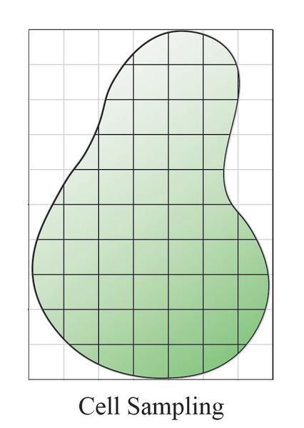
Figure 1. Samples are collected within each cell area. Cells are created by placing a uniform grid over the field boundary and sized to capture the underlying variability.
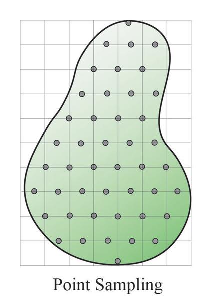
Figure 2. Samples are collected at point locations. Points are located at the intersection of grid lines (as depicted in the figure) or collected at the center of each grid cell.
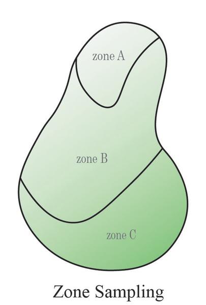
Figure 3. Samples are collected within areas of similar soil, crop, or production characteristics.
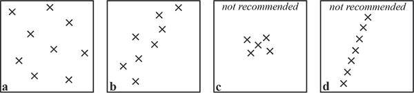
Figure 4. Cell sampling strategies include collecting (a) random soil cores within the cell or (b) systematically staggered soil cores to facilitate sampling by a vehicle. Avoid collecting soil cores in (c) clusters or (d) along straight lines.
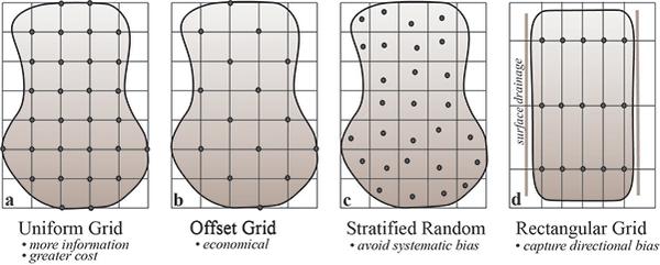
Figure 5. Point sampling designs can vary depending on the desired cost, objective, and field characteristics.
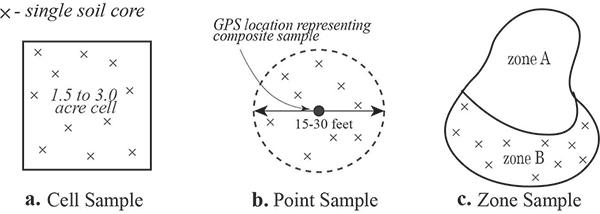
Figure 6. A composite soil sample is collected differently depending on the sampling strategy: (a) 15-20 cores within a cell (b) 8-10 cores inside a 15- to 30-foot circle around a point sample or (c) 15-20 cores inside a delineated zone within the field.
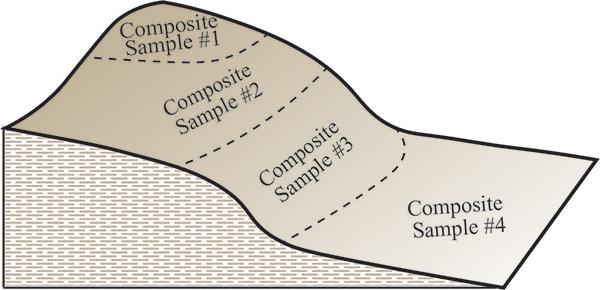
Figure 7. Example of a zone-based soil sampling approach. Zones are created and sampled to capture areas of similar production, soil, or management.
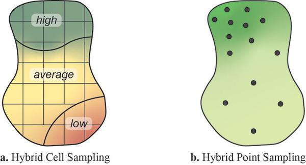
Figure 8. A hybrid approach can be applied to point or cell sampling. Hybrid approaches include (a) cells subdivided into regions with historically different productivity or (b) a greater density of point samples in areas of greater soil variability.
Costs and Benefits
Managing soils with a site-specific approach has several potential benefits. When combined with variable rate technology, site-specific management distributes nutrients and other amendments according to the spatial variation in soil properties used to determine agronomic optimum amendment rates. In site-specific management, higher rates of amendments are typically applied to locations in the field where the potential crop response is greatest, and lower rates are applied in areas less likely to respond. The desired result of a site-specific management approach is not limited to optimizing growth and yield; producers also may be aiming for increased pest and disease resistance or a better quality crop. By matching the needs and production potential of the crop to a location in the field, amendments are distributed at prescribed amounts and set to meet production goals. The approach may also have environmental benefits: though higher nutrient rates are applied in the most productive areas, reduced rates in areas where nutrients are not needed can potentially lessen the impact of nutrient runoff on water quality. Furthermore, the correction of localized nutrient deficiencies should increase nitrogen use efficiency (since other nutrients will not be limiting) and potentially reduce the risk of nitrogen runoff and leaching.
To realize the potential benefits of site-specific soil sampling and management, you must better understand yield-limiting factors within fields. Yields vary within fields for many reasons, for example, rate of rainfall, the presence or absence of weeds and insects, and existence of microclimates. All yield-limiting factors interact at various degrees with the underlying soil conditions (for example, nutrient level, pH, texture, topography, and drainage); the impact of those interactions on yield changes in both space and across time. Factors that limit yield one year may be different the next, and what is believed limiting at one location may boost production in others. Regardless, the greater the role of soil nutrient status in controlling yield, the greater the potential benefit from site-specific sampling and management.
Costs associated with site-specific sampling vary widely, depending on the services and analyses performed, and are typically associated with equipment, labor, and time. When performed in-house, much of the cost is in the initial investment and includes GPS receiver(s), an all-terrain vehicle for sample collection, and computer hardware and software required to perform the analysis. Labor and opportunity costs are also associated with learning software and developing new workflows. Increased sampling also results in extra laboratory and labor costs. The equipment and labor costs associated with variable rate equipment should also be considered.
Many agricultural consultants and equipment retailers offer precision soil sampling as a contracted service. Costs for these services can vary widely and are difficult to estimate because services are often bundled and discounted in package deals. Packages typically involve tiered pricing with offers of additional services such as tissue analysis, nematode testing, and pest or disease scouting. An informal survey of providers of precision soil sampling services in eastern North Carolina revealed costs of $6 to $10 per acre for sample collection on a 2½-acre grid cell size. Higher costs were quoted for point sampling and additional expenses related to analysis and final map production.
To justify adoption of a site-specific soil sampling and field management approach, the costs associated with increased sampling, soil analysis, and variable rate equipment and application must be offset by an increased field average yield and productivity.
Acknowledgements
The authors thank Carl Crozier and Ronnie Heiniger, the authors of Soil Sampling for Precision Farming Systems, on which this publication is based.
Publication date: Aug. 10, 2020
Reviewed/Revised: June 25, 2025
AG-439-36
N.C. Cooperative Extension prohibits discrimination and harassment regardless of age, color, disability, family and marital status, gender identity, national origin, political beliefs, race, religion, sex (including pregnancy), sexual orientation and veteran status.