
Forest harvest residue (FHR) is an important environmental component, but how do you measure it? The recent surge in interest in renewable energy in the U.S., including wood energy, has brought growing concern about the impact of biomass removal and its impact on biodiversity,
water quality, and long-term site productivity (Björheden, 2010).
Forest harvest residue can be scattered or piled. FHR usually consists primarily of material from live trees added during harvesting, such as limbs, tops, and small diameter stems and, to a lesser extent, some dead material that existed prior to harvest. In some states, biomass harvesting guidelines (BHGs) have been developed or proposed to encourage retention of forest harvest residue. Thus, assessing success of BHGs or other measures intended to mitigate environmental impacts will require sampling to determine stocking of forest harvest residue. Unlike a timber cruise, where the expense may be carried by a timber sale or management agreement, measurement of forest harvest residue is likely to be part of environmental monitoring and needs to be done quickly and inexpensively, while obtaining an acceptable level of accuracy.
Depending on the size of the residue, forest harvest residue may be referred to as coarse woody debris (CWD) or fine woody debris (FWD). For this discussion, we will refer to forest harvest residue that encompasses both CWD and FWD as defined by the USDA Forest Service. FHR also includes slash piles that are conglomerations of CWD created by human activity or natural events (Woodall and Monleon, 2007). This document will describe how to rapidly inventory scattered and piled FHR.
What Is Prism Sweep Sampling?
The prism sweep sampling (PSS) method is an accurate and efficient way to sample scattered FHR (Bebber and Thomas, 2003). This method is used to obtain volume and biomass estimates over a site when describing the spatial distribution of FHR is not needed. If you are interested in the spatial distribution of FHR over a site, it is best to use line-intercept sampling (LIS), a well-known, frequently used method employed by the USDA Forest Service Forest Inventory and Analysis Unit (Woodall and Monleon, 2007). PSS is a probability-proportional-to-size method that uses the same principles as point relascope sampling with inexpensive, readily available equipment. Woody biomass to be measured must be subtending by a prism angle where the midpoint diameter viewed from the point center is greater than the critical prism angle (Figure 1). The piece that is determined as “in” would then have its length measured.
PSS requires a clear line of sight from the point center to any potential piece of FHR. Sites with advanced herbaceous regeneration, multiple layers of FHR, or other situations where piece centers cannot be seen may require another method.
Prism-sweep and line-intercept-sampling methods were used to measure forest harvest residue within a recently harvested site in Johnston County, North Carolina, and compared with a 100 percent tally using 0.1-acre plots to compare efficiency and precision. Fifty plots were situated on a grid and of these, twenty were randomly selected for sampling. Of those twenty plots, thirteen were in a hardwood forest and seven within a pine forest. At each plot location, line-intersect, prism-sweep and 100-percent tally sampling methods were applied using a two-person crew (Tables 1 and 2).
| Sampling Design | |||
|---|---|---|---|
| Statistic | Line Intersect | Prism Sweep | 100% Tally |
| Mean | 25.97 | 21.04 | 22.32 |
| Standard Error | 3.10 | 2.51 | 1.60 |
| Median | 21.78 | 19.20 | 21.06 |
| Standard Deviation | 13.86 | 11.22 | 7.17 |
| Range | 47.66 | 45.15 | 26.11 |
| Confidence Limit (+/-) | 6.49 | 5.25 | 3.36 |
| Sampling Design | ||
|---|---|---|
| Statistic | Line Intersect | Prism Sweep |
| Mean | 17.2 | 3.2 |
| Standard Deviation | 5.4 | 1.3 |
| Range | 15 | 5 |
| Confidence Limit (+/-) | 2.5 | 0.6 |
For this field comparison, the prism sweep provided an accurate estimate when compared to the 100 percent tally of the 0.1 acre fixed-radius plots (Table 1) at a fraction of the time required for the line-intersect sampling method (Table 2).
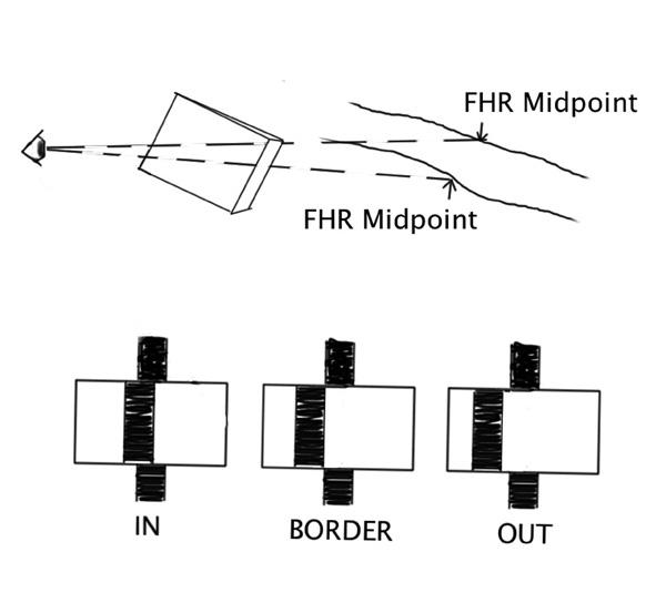
Figure 1. Sighting through a prism at the midpoint of a forest harvest residue piece to determine if it is “in” and should be sampled.
Prepare for the Inventory
Proper planning helps facilitate a successful inventory of a property. Preparation will minimize time spent in the field and increase the accuracy of the estimates determined from the inventory data.
To begin planning, you will need:
- a map or aerial photograph of the area to be sampled
- an estimate of the number of acres to be sampled
- a calculator
Before conducting the inventory, determine the number of sample points to measure and decide where they will be installed in the field. The number of points to be sampled is based on the degree of confidence desired and the variation in the amount of the FHR to be measured. You can estimate the variation in the amount of FHR from previous inventories on similar sites or by using information on the range of the observation from a small sample of the area to be measured.
The following calculation is used to determine the approximate number of points to sample.
\(n = {\left( {\frac{{S\: \bullet\: t}}{E}} \right)^2}\)
Where
n is number of sampling points that will be installed.
t is dependent on the degree of confidence required for the confidence interval; t = 1.7 for a 90% confidence interval, t = 2 for a 95% confidence interval, and t = 2.6 for a 99% confidence interval.
S is the standard deviation in the amount of the FHR to be measured. A good estimate of the standard deviation in the amount of the FHR can be determined by the range of observations from a small sample of the site to be inventoried or from a previous inventory of a similar site. To determine the standard deviation, divide the range of the observations by 4.
E is the error of tolerance, and the person who requests the inventory specifies it. E is in the same units as S.
For example: You are asked to sample a 50-acre forest tract, with an error of tolerance specified at ± 3 tons/acre and a desired confidence level set at 95 percent. A small sample of the forest tract indicates a range of 32 tons/acre of FHR. The number of sample points needed to conduct the inventory is calculated as follows.
\(S = {\textstyle{{32\:tons/ac} \over 4}} = 8\:tons/acre\)
t = 2, for a 95% confidence interval
E = ± 3 tons/acre
\(n= {\left( {{\textstyle{{S\: \bullet\: t} \over E}}} \right)^2} = {\left( {{\textstyle{{8\: \bullet\: 2} \over 3}}} \right)^2} = {\left( {{\textstyle{{16} \over 3}}} \right)^2} = 28.4 \approx 29\)
Once the number of sample points has been determined, plot their location in the field. On a map or aerial photo of the area to be inventoried, draw parallel lines that reasonably cover the tract. The lines represent the approximate path to follow in sampling. The spacing of the lines and the distance between points will be based on the sampling intensity you are trying to achieve. Draw the lines perpendicular to drainage patterns to pick up changes in vegetation caused by changes in soil moisture and elevation. Locate sample points at regular intervals, which will produce approximately the target number of sample points. Figure 2 depicts a typical layout of a sampling scheme.
It is important to understand how to navigate in the field using a compass and pacing before beginning the inventory. To learn more, read Woodland Owner Note 39, Using a Compass and Pacing.
Once the number of sample points is determined and a sampling scheme identified, you are ready to begin the inventory. The following procedure is based on a two-person team, but it can be accomplished by a single person. As with prism cruising of standing trees, a single person must return to the point center periodically between measuring lengths of “in” FHR pieces.
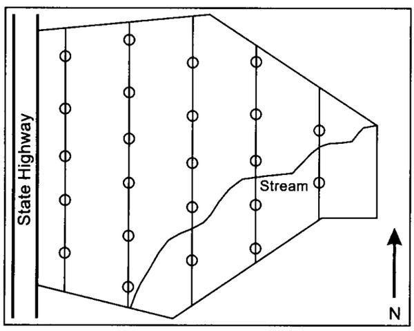
Figure 2. A typical layout of a sampling scheme.
Conduct the Inventory
To begin an inventory, you will need to gather a few pieces of equipment and locate the first sampling point center. The equipment needed for the inventory includes the following.
- BAF 10 wedge prism
- Measuring Tape (25- or 50-foot length)
- Compass
- Pin flag
- Data sheets (See examples at end of the document)
Once you have located the first sampling point, use the following guidelines to conduct the sampling of scattered FHR.
- Place a pin flag marking the sampling point.
- With the compass, determine the direction you are facing. This will be the starting and ending point as you rotate 360° around the sampling point as marked with the pin flag.
- Stand with the prism over the sampling point. Hold the prism approximately 10 inches from your eye and at a right angle to the axis of the length of the residue (Figure 1). With one eye closed, begin sighting FHR, counting only those pieces whose midpoint is offset by the prism. These pieces are considered “in” (Figure 1) and their total length is measured to the nearest inch and recorded on the data sheet. As you rotate 360o around the prism, make sure to hold the prism over the sampling point.
- After assessing scattered FHR, observe whether there is any piled FHR that has a midpoint within 24 feet of the sampling point, as marked by the pin flag. If there is a pile with a midpoint within 24 feet of the sampling point, then complete the following steps.
- Estimate the proportion of each pile that falls within 24 feet of the sampling point. The proportion is between 0 and 1 and is recorded as a decimal to the nearest tenth (0.1, 0.2, 0.3, etc.). Record this on a data sheet under the column labeled “MP.”
-
Next, estimate the packing density of each pile that falls within 24 feet of the sampling point. The proportion is between 0 and 1 and is recorded as a decimal to the nearest tenth (0.1, 0.2, 0.3, etc.). Record this on a data sheet under the column labeled “Packing Density.”
Packing density is a measure of how dense a pile of FHR is considering the amount of wood and airspace in the pile. Some examples of packing density for three different piles are shown in Figure 3. -
After determining packing density for each pile, determine the shape code that best represents the pile. Use Figure 4 to determine which shape code to use. Based on the code you select, measure the indicated dimensions. Record the dimensions and shape code under the respective columns on the data sheet.
-
Move to the next sampling point and repeat the above steps. Do this for all sampling points.
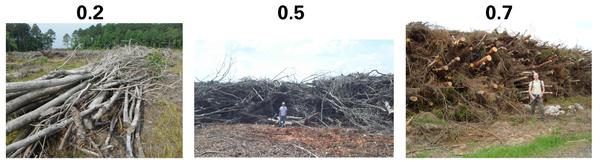
Figure 3. Packing density for three different piles.
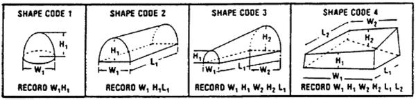
Figure 4. Shape codes and required dimensional measurements for piled FHR (Woodall and Monleon, 2007).
Calculate FHR Volume Estimate
After conducting the inventory and collecting the data, estimate the volume of scattered and piled FHR on the site using the following equations.
- Scattered FHR Volume Estimates
The cubic-foot volume of scattered FHR is calculated using the following equation based on the sum of measured lengths of tallied FHR pieces for each plot, the prism basal area factor, and number of sample points taken.
\(\bar x = {\textstyle{{\sum {L\: *\: BAF} } \over n}}\)
Where
\(\sum\)L is the sum of lengths of tallied pieces over all points,
BAF is the basal area factor of the prism used in sampling,
n is the number of sample points
After cubic feet volume is calculated for the scattered FHR, it is multiplied by a wood density value (WD) to estimate scattered FHR volume in tons per acre. The equation for this calculation is
\(\bar x = \bar x{\textstyle{{{\rm{f}}{{\rm{t}}^3}} \over {{\rm{acre}}}}} \times WD{\textstyle{{{\rm{ton}}} \over {{\rm{f}}{{\rm{t}}^3}}}}\)
where WD is constant at 0.03. This is based on the assumption that scattered FHR green weight is 60 lbs per cubic foot.
For example, measure the length of 89 “in” FHR pieces over 28 sample points. To determine which pieces were “in,” use a 10 basal area factor prism. The sum of “in” pieces measured lengths is 763 feet. With this information, the estimated cubic-foot volume of scattered FHR is
\(\bar x = {\textstyle{{\sum {L * BAF} } \over n}} = {\textstyle{{763{\textstyle{{f{t^3}} \over {acre}}} \times 10} \over {28}}} = {\textstyle{{7630{\textstyle{{f{t^3}} \over {acre}}}} \over {28}}} = 272.5{\textstyle{{f{t^3}} \over {acre}}}\)
The estimated volume of scattered FHR in tons per acre is
\(\bar x = 272.5{\textstyle{{f{t^3}} \over {acre}}} \times 0.03{\textstyle{{ton} \over {f{t^3}}}} = 8.18{\textstyle{{tons} \over {acre}}}\)
- FHR Pile Estimates
Net cubic-foot volume estimates for individual FHR piles are calculated using shape-specific formulas that incorporate height, width, and/or length measurements. Choose the formula in Table 3 based on the shape code (Figure 4) of the pile for which you are calculating volume estimates.
| Shape code | net volume equationa |
| 1 | \(\left( {{\textstyle{{\pi H{W^2}} \over 8}}} \right)\left( {PD} \right)\) |
| 2 | \(\left( {{\textstyle{{\pi HWL} \over 4}}} \right)\left( {PD} \right)\) |
| 3 | \(\left( {{\textstyle{{\pi L\left[ {\left( {{H_1}{W_1}} \right)\: +\: \sqrt {\left( {{H_1}{W_1}{H_2}{W_2}} \right)}\: +\: \left( {{H_2}{W_2}} \right)} \right]} \over {12}}}} \right)\left( {PD} \right)\) |
| 4 | \(\left[ {{\textstyle{{\left( {{L_1} + {L_2}} \right)\left( {{W_1} + {W_2}} \right)\left( {{H_1} + {H_2}} \right)} \over 8}}} \right]\left( {PD} \right)\) |
| a H,W, L refer to pile dimensions (in feet) according to shape code and PD is packing density | |
Once the net cubic-foot volume is estimated for individual piles, calculate volume per acre on a cubic-foot basis for individual sample points. This calculation is based on the sum of individual pile volume within a sample point, the sample point’s expansion factor, and the mean observed proportion of piles falling within the sample point’s plot boundary. The equation for this calculation is
\({\bar x^{pile}{\textstyle{{f{t^3}} \over {acre}}} = \sum\limits_{}^{} {{p^{plot}} \times 24 \times MP} }\)
Where
\({\sum\limits_{}^{} {{p^{plot}}} }\) is the sum of cubic-foot volume for all measured FHR piles falling within 24 feet of the sampling point,
24 is the point expansion factor, and
MP is the observed mean proportion of piles falling within 24 feet of the sampling point.
The next step is to compute the mean volume per acre of FHR piles over all sample points. This calculation is based on the sum of volume per acre for individual sample points and the number of sample points installed.
\({\bar x^{pile\: overall} = (\sum\limits_{}^{} {{p^{overall}})/n} }\)
Where
\({\sum\limits_{}^{} {{p^{overall}}} }\) is the sum of cubic-foot volume per acre of FHR piles over all sample points and
n is the number of sample points installed
After mean volume on cubic-foot-per-acre basis for piled FHR is calculated, it is multiplied by a wood density value (WD) to estimate mean volume in tons per acre for piled FHR. The equation for this calculation is
\({\overline x ^{pile\:overall} = {{\overline x }^{pile\:overall}{\textstyle{{f{t^3}} \over {acre}}} \times WD{\textstyle{{ton} \over {f{t^3}}}}}}\)
where WD is constant at 0.03. This is based on the assumption that piled FHR green weight is 60 lbs per cubic foot.
For example, assume you sampled two piles on one point over a total of 28 sample points. The shape of these piles best matches shape code 2, so you measured height, length, and width of the piles. Pile one measured 7.5 feet in height, 10 feet in length, and 5 feet in width. Pile two measured 3 feet in height, 10 feet in length, and 4 feet in width. The packing density for piles one and two is estimated at 0.6 and 0.45, respectively. The observed mean proportion of piles falling within the sample plot was 0.75. With this information, the estimated volume on a net-cubic-foot basis is
\(pile\:1 = \left( {{\textstyle{{\pi HWL} \over 4}}} \right)\left( {PD} \right)\)
\(= \left( {{\textstyle{{\pi\: \times\: 7.5\: \times\: 5\: \times\: 10} \over 4}}} \right)\left( {0.6} \right)\)
= (294.52 ft3)(0.6)
= 176.71 ft3
\(pile\:2 = \left( {{\textstyle{{\pi HWL} \over 4}}} \right)\left( {PD} \right)\)
\(= \left( {{\textstyle{{\pi\: \times\: 3\: \times\: 4\: \times\: 10} \over 4}}} \right)\left( {0.45} \right)\)
=169.64 ft3 ÷ 4
= 42.41 ft3
The cubic-foot volume for piled FHR per acre for the individual sample points is
\({\bar x^{pile} = \sum\limits_{}^{} {{p^{plot} \times 24 \times MP} }}\)
= (pile 1 + pile 2) x 24 x 0.75
\({\bar x^{pile}} = \left( {176.71{\textstyle{{f{t^3}} \over {acre}}} + 42.41{\textstyle{{f{t^3}} \over {acre}}}} \right) \times 24 \times 0.75\)
\({\bar x^{pile}} = 3944.16{\textstyle{{f{t^3}} \over {acre}}}\)
The mean cubic-foot volume over all sample points is
\({\bar x^{pile\:overall}} = {\textstyle{{\left( {\sum\limits_{}^{} {{p^{overall}}} } \right)} \over n}}\)
\(= {\textstyle{{\left( {3944.16{\textstyle{{f{t^3}} \over {acre}}}} \right)} \over {28}}}\)
\(= 140.86{\textstyle{{f{t^3}} \over {acre}}}\)
The mean volume for piled FHR in tons per acre over all sample points is
\({\bar x^{pile\:overall}} = \bar x{\textstyle{{f{t^3}} \over {acre}}} \times 0.03{\textstyle{{tons} \over {f{t^3}}}}\)
\(= 140.86{\textstyle{{f{t^3}} \over {acre}}} \times 0.03{\textstyle{{tons} \over {f{t^3}}}}\)
\(= 4.22{\textstyle{{tons} \over {acre}}}\)
Conclusion
Conducting inventories using prism-sweep sampling and fixed-radius sampling for scattered and piled FHR requires planning and several steps. Relative to other sampling methods, however, these techniques provide an excellent way to quickly conduct accurate and rapid inventories of recently harvested forests. Estimates of FHR on harvest areas can help landowners, natural-resource professionals, and others assess the success of BHGs or other measures intended to mitigate environmental impacts.
Literature Cited
Bebber, Daniel and Sean Thomas. “Prism sweeps for coarse woody debris,” Canadian Journal of Forest Research vol. 33, no. 9 (2003): 1737-1743.
Björheden, Rolf, “Efficient forest fuel supply systems: Composite report from a four year R & D programme 2007-2010.” Skogsforsk Research and Development (2010).
Woodall, Christopher and Vicente Monleon. “Sampling Protocol, Estimation, and Analysis Procedures for the Down Woody Materials Indicator of the FIA Program,” United States Department of Agriculture Forest Service General Technical Report NRS-22 (August 2007).
Publication date: May 1, 2019
Reviewed/Revised: Feb. 8, 2024
AG-754
N.C. Cooperative Extension prohibits discrimination and harassment regardless of age, color, disability, family and marital status, gender identity, national origin, political beliefs, race, religion, sex (including pregnancy), sexual orientation and veteran status.