
Introduction
While growing a crop takes substantial effort, making a profit also requires successful marketing. Some years it may be easy to profit; other years, it may be challenging. This chapter provides foundational knowledge for marketing in general, evaluation of current market conditions illustrating key price relationships, and input cost information in the form of enterprise budgets specific to North Carolina.
Marketing and price risk
Crop producers are no stranger to risk. Factors outside the producer’s control, such as weather, can influence the amount produced. Similarly, a North Carolina producer has no influence on national soybean price levels. Neither weather nor prices are perfectly predictable, and both affect producer profit and financial health—possibly for better, possibly for worse.
During a set period of time, say a year, profit will be the total revenue, less the total costs.
\(profit=total\ revenue-total\ costs\)
This section on marketing focuses on the revenue part of the equation. Total revenue will come from collecting sales of all the products a farm produces. Let’s say a farm produces corn and soybeans, then
\(profit=[(price_{soy}\times yield_{soy}\times acres_{soy}) + (price_{corn}\times yield_{corn}\times acres_{corn})] - total\ costs.\)
If we look at soybean revenue alone, we can see that price and yield are random variables—that is, we will not know the value until it occurs. We will know yield only at harvest, and we will know the price only at the time of the actual sale.
\({\underbrace{price_{soy}}_\text{unknown}}\times{\underbrace{yield_{soy}}_\text{unknown}}\times\ acres_{soy}\)
Given that producers must make input decisions—often associated with costs—before knowing prices and yields, what are the options for dealing with these unknowns?
It is easiest to address yields first. Management practices developed by crop scientists and entomologists, for example, can make soybean yields more predictable and reduce the likelihood of crop failure. In terms of financial tools, there is also crop insurance. Crop insurance can offer yield protection or revenue protection (accounting for both price and yield). The main advantages of crop insurance are that it protects against catastrophic losses and can improve producer access to credit. The disadvantages are that a premium must be paid1, and it can be complex in terms of the type and level of coverage to select.
This section is devoted to marketing and the financial tools available to manage price risk. As with yields, we ask similar questions:
- Is there anything we can do to make soybean prices more predictable?
- What can we do to reduce the financial impact of low soybean prices?
As with crop management practices, determining the “best” practices will depend on various farm characteristics—managing price risk should be specific to each farm. When choosing a price-risk management strategy, it is important to consider the producer risk tolerance and risk capacity, and national and local market conditions.
While risk tolerance and risk capacity may be related, they are separate considerations. Risk tolerance refers to the producer’s emotional ability to withstand commodity price volatility or rapidly falling prices. Someone who is risk-averse may lose sleep during times of high soybean price volatility; someone else who is risk-loving may be willing to accept exposure to soybean price fluctuations during the same volatile period. Risk capacity is the maximum amount of loss the farm enterprise can tolerate, regardless of the producer’s attitude toward risk. A farm enterprise following a good year may be capable of withstanding up to $25,000 of potential losses on soybeans; such a loss would be painful, but the farm could eventually recover. A $25,000 loss may bankrupt the same farm following a bad year.
Therefore, implementing an appropriate marketing strategy requires preparation. Mainly the producer needs to establish:
- How much potential loss am I willing to accept? [tolerance]
- What is the maximum loss the farm can withstand? [capacity]
Reviewing the broad financial picture of the farm by evaluating the cash flows, current liquidity, and profitability will help determine the answers to A and B. Since risk tolerance can exceed risk capacity, whichever one is lower, A or B, is a limit to keep in mind. The next information to establish is:
- What is the break-even price per bushel? Break-even price per acre? To find this value, we need to solve for the soybean price when profit equals zero.
\(soybean\ revenue-soybean\ costs=$0\ \rightarrow \underbrace{(price_{soy}\times yield_{soy}\times acres_{soy})}_\text{soybean revenue} = soybean\ costs\)
This can be rearranged as:
\(price_{soy}^{breakeven}\ =\ {{soybean\ costs}\over{yield_{soy}}\ \times\ {acres_{soy}}}\)
- At what price will you meet the loss limit determined in steps A and B? Say the loss limit is $X ; then at what price per bushel, and per acre, is the loss limit reached? The process is very similar to finding the break-even price.
\(soybean\ revenue-soybean\ costs=-\ $X \\ \rightarrow\ soybean\ revenue=soybean\ costs-\$X\\ \rightarrow\ {\underbrace{\left(price_{soy}\times yield_{soy}\times acres_{soy}\right)}_\text{soybean revenue}}=soybean\ costs-$X\)
Which can also be rearranged as:
\({price}_{soy}^{loss\ limit}=\frac{soybean\ costs-$X}{yield_{soy}\times acres_{soy}}\)
Steps C and D require budgets because costs are needed to solve for the break-even and loss-limit prices (enterprise budgets are provided at the end of this chapter). The steps also require making an informed assumption about yield. Finally, the number of acres planted must be decided. Deciding on the number of acres to plant before knowing prices and yields is difficult when multiple crops compete for acreage (an example might be corn and soybeans). Consequently, these limits may need to be revisited and revised during the planning stages.
Steps C and D can be thought of as determining which guard rails to set up. The revenue guard rails can be set up using crop insurance OR a combination of crop insurance and hedging strategies. Beyond these guard rails, you can determine the prices needed to meet other profit objectives, if desired.
Soybean Prices in North Carolina
A common set of tools to manage price risk is given in the next subsection. To use these tools appropriately, it is important to understand how prices in North Carolina will be related to national soybean prices.
The Chicago futures price, which we think of as the national soybean price, is a contract in which a buyer and seller agree to a price for a standard quantity of soybeans that will be exchanged at some future date. The futures price adjusts frequently depending on national supply and national demand. National storage stocks and national acres and yield make up the total U.S. soybean supply. Midwestern states, such as Illinois, Iowa, and Minnesota, produce the most soybeans in the U.S. These states are physically closer to future market delivery locations in Chicago. In addition, these Midwest sources are export-oriented, given their advantageous proximity to the Mississippi River. Therefore national prices will adjust with national supply, which depends largely on the market conditions in the Midwest.
North Carolina markets are different. North Carolina is not close to Chicago; rail is the primary link between North Carolina markets and Chicago and national markets. Also, North Carolina is a net importing region due to a large livestock industry located in the state. In addition to what is happening nationally, North Carolina supply and demand conditions can significantly impact the price North Carolina producers receive. Thus, North Carolina conditions are important to consider as part of price risk.
The primary measure linking local North Carolina prices to futures prices is “basis.”
\(basis={\underbrace{cash\ price}_\text{current price received in NC}}-{\underbrace{futures\ price}_\text{known as the national price} }\)
Rearranged,
\(cash\ price=futures\ price+\ {\underbrace{basis}_\text{reflects relative NC conditions}}\)
Figure 2-1 compares the North Carolina cash price to the nearby Chicago futures price, showing that the relationship between these two price series adjusts over time and that basis can be positive or negative.
Unfortunately, the basis equation is deceptive in its simplicity. Futures contracts are very specific to product quality, delivery location, and time of delivery. The hidden feature of basis is that it combines two types of price relationships: (1) prices today and the futures contract delivery date, and (2) prices in North Carolina and futures contract delivery locations. Typically, the basis is reported using the nearby futures contract, that is, the futures contract set to expire next. Futures contracts are very specific, and prices are quoted for listed grades/quality, so this will also affect the price received.
When thinking about North Carolina basis in general, there are a few assumptions to work from, which are usually, but not always, true.
- The basis is more predictable than the total cash price.
- End users, such as a crushing facility, will have a higher basis than an intermediary handler.
- Basis varies throughout the year and is lowest at harvest.
This NC State Extension web page provides regular updates on historical price and basis data for many North Carolina locations, shown in Figure 2-2. The CME Group website provides futures prices. These data can be used to compare current offers to historical prices and basis levels.
This section has emphasized that North Carolina prices are composed of two components that potentially should be included as part of a price-risk management strategy. A complete price-risk management strategy will consider if and how to manage basis, if and how to manage the futures price, or both.
Hedging
The marketing cross is a framework that can help map out a price-risk management strategy. The cross is shown in Figure 2-3 and suggests hedging strategies to use based on both national and North Carolina market conditions.2
More information about each strategy follows, but it is important to stress that hedging is not free. There may be apparent costs, such as fees, associated with a particular strategy. Non-obvious costs can include time spent monitoring markets and managing one’s position. And some methods can limit the producer’s ability to gain from price increases. In general, hedging aims to reduce or eliminate the impact of falling soybean prices—the goal is not necessarily to maximize the soybean price.
In addition, the prescribed strategies do not specify how much to hedge and when to hedge. Typically, zero to 60% of expected production is hedged. A natural time to place a hedge is at or after planting, once a reasonable expectation of production can be formed. But hedges can be placed any time. Someone may place a hedge at a particular time to secure advantageous soybean prices or because the farm financial circumstances have changed. Having the farm-specific guard rails and price objectives in mind will guide these decisions as situations evolve.
Using futures and options
Futures and options are used to manage national price risk.
Hedging with futures: To initiate a futures hedge, one sells soybean futures (in other words, goes “short") for the contract expiring just after harvesttime. Then at harvest, when delivering to a local buyer for the cash price, exits the futures market by buying soybean futures (in other words, goes “long”).
Per bushel outcome on hedged production
\({\underbrace{cash\ price\ }_\text{received from local buyer}}+\ \underbrace{ (futures\ sell\ price\ –\ futures\ buy\ price)}_\text{futures market profit or loss}\)
Important to note:
Because a futures contract is an agreement to buy or sell in the future, a margin deposit representing a fraction of the total contract value is required. The deposit is required for both buyers and sellers. From then on, the entire gains and losses from day-to-day price changes are reflected in the margin account. If a margin account balance falls below a certain level, the producer will receive a margin call, which is a notice from the broker to deposit additional cash into the account immediately. This process is part of the safeguards to ensure the financial integrity of futures contracts. However, someone should always have cash on hand while the futures position is open, which may not be feasible for everyone.
Another obstacle for producers is that a futures contract, which is for 5,000 bushels, may be too large (or too lumpy) of a quantity to hedge, depending on the farm’s expected soybean production. Smaller-sized futures contracts of 1,000 bushels called “minis” are available. However, minis tend to have lower trading activity levels than standard-sized contracts, which can adversely impact liquidity and the ability to exit and enter the market.
Hedging with options: To initiate a hedge using options, the producer should buy "put" options on the soybean futures contract that expire just after harvesttime. A put option gives the holder the right to sell a futures contract at a specific price called the strike price. The fee for this right is called the option premium.
Per bushel outcome on hedged production
In this case, the outcome depends on how the futures price and strike price compare at harvest time. If the futures price > strike price then the put option expires.
\(cash\ price\ –\ put\ premium\)
However, if futures price< strike price, then someone can buy a futures contract at the current market price and exercise the put option to sell at the strike price.
\(cash\ price\ –\ put\ premium+({\underbrace{futures\ sell\ price}_\text{put option strike price}}-futures\ buy\ price)\)
Important note:
Options are not available on the mini-sized futures contracts. But, unlike futures, buying an option does not require maintaining a margin account.
Contracting with a local buyer
The only way to manage basis risk is to contract with a local buyer. However, local buyers often offer contracts with means of managing national price risk. There are endless ways to design these contracts, including incorporating futures markets, and they can quickly become complex. Two of the more straightforward and commonly used contract types are discussed below.
Hedging with a cash forward contract: Make an agreement with a local buyer for the total price they will pay per bushel upon delivery during harvest. Since the total price per bushel is agreed upon, fluctuations in the futures price and basis are no longer relevant for the quantity hedged.
Per bushel outcome on hedged production
\(forward\ contract\ price\)
Important note:
In this case, both national price and basis risk are transferred from the producer to the local buyer. Because of this, local contracts can have service fees or built-in risk premiums. And because a local custom contract is not traded on an exchange, futures market structures to easily enforce the contract and provide flexibility to exit the contract early are unavailable.
Hedging with a basis contract: Make an agreement with a local buyer for the basis they will pay per bushel upon delivery during harvest. This locks in basis but leaves someone exposed to fluctuations in the futures price.
Per bushel outcome on hedged production
\(futures\ price+contract\ basis\)
Important note:
In this case, only basis risk is transferred from the producer to the local buyer. These contracts may also include service fees or built-in risk premiums.
Table 2-1. Summary of Marketing Cross Strategies
|
Marketing Strategy |
Exposed to Futures Price Risk? |
Exposed to Basis Risk? |
Important to Note |
|
Do Nothing (for example, cash sale at harvest) |
Yes |
Yes |
|
|
Cash Forward Contract |
No |
No |
|
|
Basis Contract |
Yes |
No |
|
|
Futures Hedge |
No |
Yes |
|
|
Put Options Hedge |
Yes, but limited |
Yes |
|
Footnotes
1Crop insurance premiums are subsidized by the Federal Crop Insurance Corporation (FCIC), so farmers do not pay the full cost of insurance.↵
2Piggott, N.E. G.A. Shumaker, and C.E. Curtis. 2005. “A Guide to Price Risk Management in Grain Marketing for North Carolina, South Carolina, and Georgia” (PDF, 2.4 MB).↵
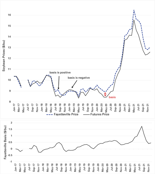
Figure 2-1. Fayetteville Versus Nearby Chicago Futures Prices
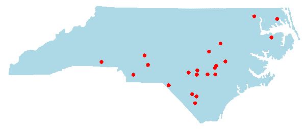
Figure 2-2. Locations with Historical Price and Basis Data
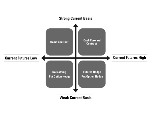
Figure 2-3. The Marketing Cross
Outlook for 2022 and beyond
This section discusses the supply and demand conditions both in North Carolina and nationally. The relationship between supply and demand trends and prices is highlighted—providing context in which to develop a marketing and risk-management strategy. Outlook factors discussed here are time-sensitive and become outdated. The following discussion highlights some essential concepts about expectations and essential relationships in play moving into a new crop year.
North Carolina Soybean Production
Over the past five years (2016 to 2020), the North Carolina soybean crop has averaged around $557 million, and in a good year, the crop is worth as much as $674 million to farmers (2020). North Carolina farmers have planted an average of 1.628 million acres of soybeans over the past five years (2017 to 2021) (Table 2-2). Soybeans have the most significant footprint in row crop acres in North Carolina, and most soybean acres in North Carolina are in the eastern part of the state in the coastal plain. Leading soybean counties in 2021, based on planted acres, include Robeson, Union, Beaufort, Pitt, Sampson, Wayne, and Duplin. The most recent five-year (2017 to 2021) average production is 59.574 million bushels, with an average yield of 37.2 bushels per acre over the same period (Table 2-2). The five-year (2016 to 2020) marketing year average price is $9.52 dollars per bushel (Table 2-2). A final important component of North Carolina soybean production accounts for a small share of national production, explaining why soybean production in North Carolina has minimal influence on prices nationally. For example, in 2021, North Carolina’s share of national production was 1.4% (65.6/4,435—North Carolina bushels over total bushels produced nationally).
In 2021, North Carolina farmers planted 1.650 million acres of soybeans that represented a turnaround in acreage, which had been on the decline over the past four years from the most recent high of 1.820 million acres in 2015 (see Table 2-2 and graph in Figure 2-4[a]). With favorable growing conditions in 2021, the average yield was a record 40 bushels per acre, equaling previous highs in 2014 and 2017 (see Table 2-2 and graph in Figure 2-4[b]). Planted acres and record yields in 2021 culminated in the third-largest harvest, 65.6 million bushels (the record was 69.2 million in 2014) (Figure 2-4[c]). As of this publication date (January 2022), the 2021 marketing year average had not been determined. However, prices in 2021 have been higher than previous years' $11.20 per bushel; the monthly average for soybeans for September to December across locations has been $12.33 per bushel (YTD), which is less than the previous high of $14.00 per bushel in 2012 (Figure 2-4[d]). Suppose prices remain strong for the remainder of the 2021 to 2022 marketing year. In that case, North Carolina soybean growers will see receipts exceeding $800 million ($12.33 per bushel × 65.6 million bushels = $808 million) for their 2021 crop, which will be the second highest on record below the previous high of $874 million set in 2012.
Table 2-2. North Carolina Soybean Acres, Yields, and Production 2000 to 2021
| Year | Acres Planted |
Acres Harvested |
Yield (Bu/Acre) |
Production (Mill Bu) |
Price (Marketing Year) ($/Bu) |
Production (Mill $) |
|---|---|---|---|---|---|---|
|
2000 |
1,400,000 |
1,360,000 |
32.5 |
44.200 |
4.51 |
199 |
|
2001 |
1,380,000 |
1,350,000 |
32.0 |
43.200 |
4.29 |
185 |
|
2002 |
1,370,000 |
1,290,000 |
24.0 |
30.960 |
5.63 |
174 |
|
2003 |
1,450,000 |
1,400,000 |
30.0 |
42.000 |
7.29 |
306 |
|
2004 |
1,530,000 |
1,500,000 |
34.0 |
51.000 |
5.56 |
284 |
|
2005 |
1,490,000 |
1,460,000 |
27.0 |
39.420 |
5.64 |
222 |
|
2006 |
1,370,000 |
1,360,000 |
32.0 |
43.520 |
6.35 |
276 |
|
2007 |
1,440,000 |
1,380,000 |
22.0 |
30.360 |
10.10 |
307 |
|
2008 |
1,690,000 |
1,670,000 |
33.0 |
55.110 |
9.33 |
514 |
|
2009 |
1,800,000 |
1,750,000 |
34.0 |
59.500 |
9.59 |
571 |
|
2010 |
1,580,000 |
1,550,000 |
26.0 |
40.300 |
12.00 |
484 |
|
2011 |
1,380,000 |
1,360,000 |
30.5 |
41.480 |
12.10 |
502 |
|
2012 |
1,590,000 |
1,580,000 |
39.5 |
62.410 |
14.00 |
874 |
|
2013 |
1,480,000 |
1,450,000 |
33.5 |
48.575 |
13.10 |
636 |
|
2014 |
1,750,000 |
1,730,000 |
40.0 |
69.200 |
10.20 |
706 |
|
2015 |
1,820,000 |
1,730,000 |
32.0 |
55.360 |
8.68 |
481 |
|
2016 |
1,690,000 |
1,660,000 |
35.0 |
58.100 |
9.80 |
569 |
|
2017 |
1,700,000 |
1,690,000 |
40.0 |
67.600 |
9.50 |
642 |
|
2018 |
1,650,000 |
1,570,000 |
33.0 |
51.810 |
8.66 |
449 |
|
2019 |
1,540,000 |
1,520,000 |
35.0 |
53.200 |
8.71 |
463 |
|
2020 |
1,600,000 |
1,570,000 |
38.0 |
59.660 |
11.20 |
674 |
|
2021 |
1,650,000 |
1,640,000 |
40.0 |
65.600 |
||
|
Average |
1,628,000 |
1,598,000 |
37.2 |
59.574 |
9.52 |
557 |
|
Average |
1,561,364 |
1,525,909 |
32.9 |
50.571 |
8.87 |
453 |
|
Min |
1,370,000 |
1,290,000 |
22.0 |
30.360 |
4.29 |
174 |
|
Max |
1,820,000 |
1,750,000 |
40.0 |
69.200 |
14.00 |
874 |
Source: USDA/NASS Quick Stats (Accessed January 2022)
The four graphs in Figure 2-4—acres, yields, production, and price—reveal upward trends over 2000 to 2021 for all four factors of production. The year 2021 was a below-trend year for acreage but a turnaround from previous years. Suppose this turnaround continues in 2022, with favorable planting conditions and strong new crop prices. In that case, planted acreage should return to above-trend levels and approach previous highs above the 1.8 million acreage level. With 2021 being a record yield year and a recent typical sawtooth pattern in yields with back-to-back increases in yields being less common (recent exceptions have been 2021, 2020, 2017, 2012, and 2009), it remains to be seen whether yields can go higher in 2022. If yields do go higher in 2022, this would be the first time that back-to-back increases have occurred for four years running—2019, 2020, 2021, and 2022—at least dating back to 2000. The growing conditions in 2022 will be a crucial driver for whether yields can be record level in 2022. If favorable growing conditions eventuate in 2022 and with the above-trend planted acreage, then expectations should be for a crop that will test the previous high of 69.2 million bushels in 2014. A record level of production in 2022, combined with higher prices in 2022 projected in the range of $12.80 to $13.30 (2022 November futures are trading at $13.15 per bushel at the time of this writing in January 2022, and new crop soybean basis in January are averaging about -$0.35 to $0.20 per bushel for an estimate of 2022 price of $12.80 to $13.30 per bushel), leads to a projection of receipts in 2022 exceeding $840 million and close to the record cash receipts of $874 million set in 2012. Of course, it is impossible to predict such things so far in advance, but if there are favorable conditions at planting time and promising new crop futures on offer, this may entice producers to plant significant acreage of soybeans in 2022. With favorable growing conditions in 2022, the upcoming year promises to be a record or near-record year for North Carolina soybean production and receipts.
U.S. Soybean Situation and Outlook
Table 2-3 shows several highlights concerning the current demand and supply of U.S. soybeans and the outlook for U.S. soybean markets moving into 2022. The national soybean crop in 2021 was 5.2% higher than the previous year’s crop, with a total production of 4.435 billion bushels. The higher production level resulted from an increase in acreage to 97.2 million acres (an increase of 4.6% from 2020) and a slight gain in yields to 51.4 bushels per acres (an increase of 0.8% from 2020). The 51.4-bushel yield in 2021 was a trend yield and was only 0.5 bushels from the record yield set in 2016. The planted acreage of 87.2 million acres was 3 million acres below the record level set in 2017. With demand having been strong and outstripping production the previous two years and depleting stocks, a mere 257 million bushels of beginning stocks rounded out the estimated 2021/22 marketing year supply of 4.707 billion bushels.
Table 2-3. USDA Supply/Demand Balance Sheet for Soybeans
|
Category |
Item/Use |
2019/20 |
2020/21 Est |
2021/22 Proj |
%Δ 2021/22 |
|---|---|---|---|---|---|
|
Production Acreage |
Acres Planted (millions of acres) |
76.1 |
83.4 |
87.2 |
4.6 |
|
Acres Harvested (millions of acres) |
74.9 |
82.6 |
86.3 |
4.5 |
|
|
Bu/Harvested Acre (millions of acres) |
47.4 |
51.0 |
51.4 |
0.8 |
|
|
Supply |
Beginning Stocks |
909 |
525 |
257 |
-51.0 |
|
Production |
3,552 |
4,216 |
4,435 |
5.2 |
|
|
Total Supply |
4,476 |
4,761 |
4,707 |
-1.1 |
|
|
Use |
Crushing |
2,165 |
2,141 |
2,190 |
2.3 |
|
Exports |
1,679 |
2,265 |
2,050 |
-9.5 |
|
|
Seed and Residuals |
108 |
97 |
102 |
5.2 |
|
|
Total Use (Demand) |
3,952 |
4,504 |
4,357 |
-3.3 |
|
|
Stocks |
Ending Stocks |
525 |
256 |
350 |
36.7 |
|
Ending Stocks, % of Use |
13.3 |
5.7 |
8.0 |
41.3 |
|
|
Pricing |
U.S. Season Average Farm |
$8.57 |
$10.80 |
$12.60 |
16.7 |
|
Price, $/ Bu |
Source: World Agricultural Supply and Demand Estimates (WASDE), USDA, January 2022
Total demand in 2021 remained strong, with a record domestic crush of 2,190 million bushels and strong exports of 2.050 billion bushels (which is only 215 million bushels below the record 2,265 million bushels set the year before), for a total use of 4.357 billion bushels, which is 147 million bushels shy of the total record use of 4.504 billion bushels set in 2020. Domestic crush demand has been strong, as evidenced by this record of 2.190 billion bushels in 2021, even despite prices being considerably higher, having increased 16.7% over the previous year, or $1.80 per bushel. Export demand softened and declined 9.5% from the previous year due to the higher prices. The combined domestic crush and export demand rounded out the total use estimated at 4.357 billion bushels for 2021/22.
With production in 2021 slightly outstripping demand (which has not been the case for the previous two years), as illustrated in Figure 2-5, there is an estimated increase in ending stocks of 36.7%, with ending stocks estimated to be 350 million bushels. Figure 2-5 illustrates that the market, in response to back-to-back years of demand outstripping supply and depleted ending stocks, higher prices in 2021 rationed demand, which—combined with 5.2% production increase—brought some relief for ending stocks in 2021/22. With ending stocks estimated to be 350 million bushels in 2021/22, this is still 162 million bushels below the previous five-year (2016-2020) average of 512 million. These stock levels going into 2022 are slightly better than the previous year, being 93 million bushels higher. The soybean ending stock situation is still considerably tight. In 2022, if the U.S. planted and harvested the same levels as 2021, zero carryout would occur if a 350/860.3=4.05 bushels per acre yield loss—or about 7.8% of the expected trend yield of 51.9 bushels per acre—occurred. This tightness in stocks combined with the uncertainty for growing conditions in 2022 provides some support to new crop soybean prices. In addition, support for new crop soybean prices also stems from soybean acres competing with corn acreages in the following months in a bid for acres in 2022.
New crop soybean prices for 2022 (the November 2022 futures contract price) as of this writing (January 2022) closed at $13.151/2 on the week ending January 21, 2022. This futures contract has been trading in an upward trend since early December 2021 when it was about $12.00 per bushel, having gained $1.15 per bushel since then. It is noteworthy that soybeans and corn will compete for acreage in 2022. Over the coming months, the new crop corn contract for 2022 (the December 2022 futures contract price) had also increased since early December 2021, when it was about $5.40 per bushel, and is now trading around $5.65 per bushel, a gain of $0.25 per bushel. The longer-term new crop soybean-corn ratio is 2:4, and so the current ratio of 2:3 (13.15/5.65) provides a slight advantage for farmers favoring corn acres over soybean acres in 2022. Comparing the tightness of stocks to soybeans and corn, with soybeans at 8% and corn at 10.4%, we might have expected this new crop soybean-corn ratio to be higher than it is. This is perhaps a signal that new crop soybean futures will continue to strengthen more significantly than corn as per the past few months, as soybeans position for an increase in acreage to further replenish stocks in 2022. As it stands, the current demand and supply situation in early 2022 is promising for soybean producers, with the momentum in favor of higher planted acres and higher prices. If growing conditions are favorable and the weather cooperates, the stage is set for record production or near-record production at profitable price levels. It should also further replenish stocks to a more comfortable level of about 500 million bushels.
A final significant concern coming into the 2022 crop year and planning period is the uncertainty about profitability in 2022 due to significantly increased production costs. In the next section, which focuses on enterprise budgets, this increase in some of the significant input costs is apparent, compared to previous years. For example, critical inputs for soybean production have increased in cost from the previous year in 2021, such as potash (over 200%) and herbicides (32%). These increased costs are harmful to profit and need to be factored into planting and marketing decisions. Recall the importance of soybean costs in calculation of the break-even and loss limit prices.
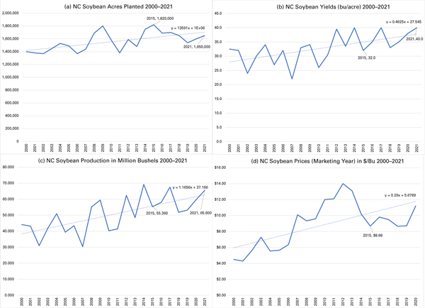
Figure 2-4. North Carolina Soybean Acres, Yields, Production, and Price
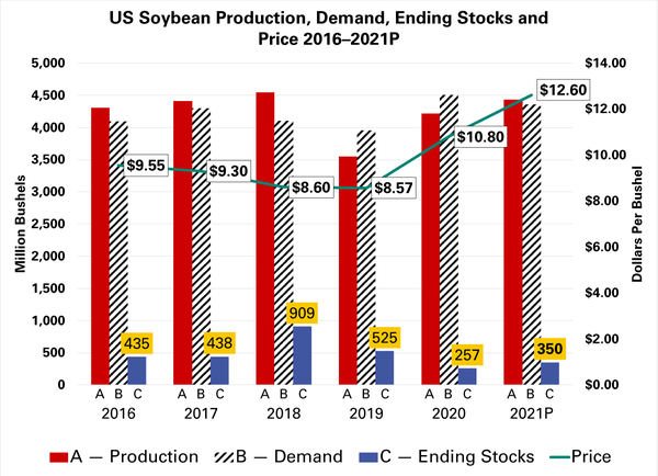
Figure 2-5. U.S. Soybean Production, Demand, Ending Stocks, and Price 2016-2021P
Enterprise Budgets
Labor, November 12, 2021
There were initial indications in 2020 that the H2A Adverse Effect Wage Rate would stay frozen through 2022 because of the pandemic. The reported hourly rate for H2A, Non-Range Occupants, effective Feb. 23, 2021, for North Carolina was $13.15, an increase from the 2020 wage rate of $12.67, according to the U.S. Department of Labor. Previous studies conducted in 2016 by NC State ARE determined that there are additional fixed costs associated with hiring H2A labor, such as provision of housing, workers compensation, transportation, utilities, and growers association fees. This cost can bring the total hourly rate of H2A to an additional $2 to $3—or more, depending on your farm’s labor efficiency. There is speculation that the H2A rate will increase by another $1 to $1.50 in 2022. It would be wise to assume that the labor shortages due to a post-pandemic economy will only complicate an already difficult labor market in the agricultural sector, regardless of the source of labor.
In the “Variable Costs” section under the line item of the budgets (Tables 2-5 to 2-9) titled “Tractor/Machinery” is the assumed variable cost for listed equipment. That equipment list, along with the associated cost, can be found under the “Per Acre Machinery and Labor Requirements” section of the budget. The labor hours are included and listed in this section and assumes the $13.15 per hour rate plus an additional 15% inefficiency rate for employees operating equipment. This is meant to account for time between fields, daily maintenance, and equipment logistics.
Interest Rates, November 12, 2021
In February 2021, the U.S. Department of Agriculture announced lending rates of 1.375% for Farm Service Agency farm-operating loans. Private banks are offering terms from 1.1% to 2.5% based on good credit and business history. Actual interest rates can vary based on the purpose of the loan and the individual famer. Rates can start as high as 12% for unique lending options and/or poor or no credit history. The 2022 budgets have an assumed 2% interest for operational loans supporting the cost of seed, pest control, fuel, electricity, irrigation, cover crop, equipment maintenance, and labor (where applicable) across all budgets. For equipment, loans, and other long-term loans, current rates vary from 2.5% to 6.9%, depending on the terms and amount of the loan. We assume a 5-year loan fixed rate at 2.9%. All indications now show a stable rate through spring of 2022 prior to planting. Because of the decrease in rates of long-term equipment loans, there is a decrease in Tractor/Machinery fixed costs in the budgets, as compared to 2021.
Energy Cost, November 12, 2021
The U.S. Energy Information Administration predicted increases across the board, effective Oct. 13, 2021. Its estimations for the U.S. in 2022 are:
- Propane increase: 54%
- Heating oil increase: 43%
- Natural gas increase: 30%
- Electricity increase: 6%
The National Oceanic and Atmospheric Administration is predicting heating degree-days to be 3% higher this year than last year for the nation, and even if the winter is warmer than average, energy cost is expected to increase. Farm use of propane in North Carolina averaged $1.99 per gallon as of Oct. 15, 2021. Propane for tobacco is mainly used in the summer months, when demand is low. Futures markets show a 28% decrease in price for liquid propane (LP) from October to the summer months, when LP will be used on the farm, a normal decrease based on demand. The budgets apply the seasonal price decrease of LP to assume an average cost of $1.43 per gallon July through August. This is roughly a 30% increase from seasonal low LP prices in 2021. Statewide gas prices in North Carolina averaged 3.21 as of Oct. 21, 2021. Since October 2020, North Carolina experienced a $1.20 per gallon increase overall. Gas prices are set at $3.20 in the 2022 budgets.
U.S diesel prices have increased $0.50 since May, 2021, to $3.67 per gal. As of Oct. 18, 2021, North Carolina average on-road diesel prices are estimated to be $3.50. The N.C. Department of Agriculture and Consumer Services (NCDA&CS) production cost report (Table 2-4) shows an average of $2.86 per gallon for farm diesel fuel, with a range of $0.14. U.S. diesel futures look relatively stable through 2022, with an expected mild decrease in price. The rate for farm diesel in the budgets is set at $2.80. This is a significant increase from cost indicated in the 2021 budgets, roughly 120%. Because of an increase in the price of farm-use diesel fuel, there is an increase in the Tractor/Machinery variable costs listed in all the budgets in 2022 as compared to 2021.
Fertilizer Cost
Table 2-4. The NCDA&CS Production Cost Report Prices as of 11/24/2021
|
Product |
Offer |
Average |
|---|---|---|
|
18-46-0 |
649.00-1,082.00 |
818.13 |
|
18-46-0, Bulk |
.00-1,042.00 |
778.13 |
|
10-10-10 |
410.00-595.00 |
505.67 |
|
10-10-10, Bulk |
370.00-555.00 |
465.67 |
|
Lime |
.00-250.00 |
222.83 |
|
Lime, Spread |
36.50-65.00 |
52.38 |
|
Potash |
740.00-1,029.00 |
858.50 |
|
Potash, Bulk |
700.00-989.00 |
818.50 |
|
Calcium Nitrate |
495.00-597.00 |
532.33 |
|
Liquid Nitrogen 30-32% |
350.00-750.00 |
511.25 |
|
Urea, Bulk |
447.00-1,015.00 |
704.00 |
|
Ammonium Sulfate |
452.00-652.00 |
521.33 |
|
Ammonium Sulfate, Bulk |
385.00-612.00 |
457.25 |
|
Whole Cottonseed |
220.00-230.00 |
226.25 |
Based on 2021 for fertilizer products used in the budgets, the percentage multiplier for the increase in cost is: 2021 cost × % Multiplier = 2022. Examples:
- 18-46-0 (DAP) = 162%
- 10-10-10 = 140%
- Lime = 0%
- Potash (0-0-60) = 203%
- Calcium Nitrate (15-0-0) = 102%
- Liquid Nitrogen (30-0-0) = 182%
- Urea (46-0-0) = 135%
Budget Tables
Table 2-5. Soybean Conventional 2022 — 50 Bushel Actual Yield
Estimated Costs and Returns Per Acre for High Maintenance Soybeans
|
Categore |
Item |
UNIT |
QUANTITY |
PRICE OR COST/UNIT |
TOTAL PER ACRE |
YOUR FARM |
|---|---|---|---|---|---|---|
|
1. GROSS |
SOYBEANS |
BU. |
50 |
$12.51 |
$625.50 |
|
|
TOTAL RECEIPTS: |
$625.50 |
|||||
|
2. VARIABLE |
SEED (CERTIFIED) |
THOU. |
110 |
$0.40 |
$44.00 |
|
|
FERTILIZER, PHOSPHATE (0-46-0) |
LBS |
87 |
$0.26 |
$22.61 |
||
|
FERTILIZER, POTASH (0-0-60) |
LBS |
123 |
$0.43 |
$53.03 |
||
|
LIME (PRORATED) |
TON |
0.33 |
$54.50 |
$17.99 |
||
|
HERBICIDES |
ACRE |
1 |
$47.36 |
$47.36 |
||
|
INSECTICIDES |
ACRE |
1 |
$3.96 |
$3.96 |
||
|
FUNGICIDES |
ACRE |
1 |
$25.07 |
$25.07 |
||
|
SURFACTANT |
ACRE |
1 |
$3.82 |
$3.82 |
||
|
AERIAL APPLICATION |
APPL |
0 |
|
|
||
|
HAULING |
BU. |
50 |
$0.26 |
$13.00 |
||
|
TRACTOR/MACHINERY |
ACRE |
1 |
$34.40 |
$34.40 |
||
|
LABOR |
HRS |
2.14 |
$13.15 |
$28.14 |
||
|
SCOUT |
ACRE |
1 |
$12.00 |
$12.00 |
||
|
INTEREST ON OP. CAP. |
DOL. |
$110.88 |
2.0% |
$2.52 |
||
|
TOTAL VARIABLE COSTS: |
$307.90 |
|||||
|
3. INCOME ABOVE VARIABLE COSTS: |
$317.60 |
|||||
|
4. FIXED |
TRACTOR/MACHINERY |
ACRE |
1 |
$74.26 |
$74.26 |
|
|
TOTAL FIXED COSTS: |
$74.28 |
|||||
|
5. OTHER |
GENERAL OVERHEAD |
DOL. |
$307.90 |
7.0% |
$21.55 |
|
|
TOTAL OTHER COSTS: |
$21.55 |
|||||
|
6. TOTAL COSTS: |
$403.73 |
|||||
|
7. NET RETURNS TO LAND, RISK, AND MANAGEMENT: |
$221.77 |
|||||
Break-Even Yield
Variable costs: 25 bu.Total costs: 32 bu.
Break-Even Price
Variable costs: $6.16
Total costs: $8.07
Table 2-6. Soybean Conventional 2022 — 42 Bushel Actual Yield
Estimated Costs and Returns Per Acre for Mid Maintenance Soybeans
|
Category |
Item |
UNIT |
QUANTITY |
PRICE OR COST/UNIT |
TOTAL PER ACRE |
YOUR FARM |
|---|---|---|---|---|---|---|
|
1. GROSS |
SOYBEANS |
BU. |
42 |
$12.51 |
$525.42 |
|
|
TOTAL RECEIPTS: |
$525.42 |
|||||
|
2. VARIABLE |
SEED (CERTIFIED) |
THOU. |
110 |
$0.40 |
$44.00 |
|
|
FERTILIZER, PHOSPHATE (0-46-0) |
LBS |
73 |
$0.26 |
$18.99 |
||
|
FERTILIZER, POTASH (0-0-60) |
LBS |
104 |
$0.43 |
$44.55 |
||
|
LIME (PRORATED) |
TON |
0.33 |
$54.50 |
$17.99 |
||
|
HERBICIDES |
ACRE |
1 |
$44.37 |
$44.37 |
||
|
INSECTICIDES |
ACRE |
0 |
|
|
||
|
FUNGICIDES |
ACRE |
1 |
$12.53 |
$12.53 |
||
|
SURFACTANT |
ACRE |
1 |
$2.85 |
$2.85 |
||
|
AERIAL APPLICATION |
APPL |
0 |
$ - |
$ - |
||
|
HAULING |
BU. |
42 |
$0.26 |
$10.92 |
||
|
TRACTOR/MACHINERY |
ACRE |
1 |
$33.64 |
$33.64 |
||
|
LABOR |
HRS |
2.05 |
$13.15 |
$26.96 |
||
|
SCOUT |
ACRE |
1 |
$12.00 |
$12.00 |
||
|
INTEREST ON OP. CAP. |
DOL. |
$102.88 |
2.0% |
$2.19 |
||
|
TOTAL VARIABLE COSTS: |
$270.99 |
|||||
|
3. INCOME ABOVE VARIABLE COSTS: |
$254.43 |
|||||
|
4. FIXED |
TRACTOR/MACHINERY |
ACRE |
1 |
$67.51 |
$67.51 |
|
|
TOTAL FIXED COSTS: |
$67.51 |
|||||
|
5. OTHER |
GENERAL OVERHEAD |
DOL. |
$270.99 |
7.0% |
$18.97 |
|
|
TOTAL OTHER COSTS: |
$18.97 |
|||||
|
6. TOTAL COSTS: |
$357.47 |
|||||
|
7. NET RETURNS TO LAND, RISK, AND MANAGEMENT: |
$167.95 |
|||||
Break-Even Yield
Variable costs: 22 bu.
Total costs: 29 bu.
Break-Even Price
Variable costs: $6.45
Total costs: $8.51
Table 2-7. Soybean Conventional 2022 — 35 Bushel Actual Yield
Estimated Costs and Returns Per Acre for Low Maintenance Soybeans
|
Category |
Item |
UNIT |
QUANTITY |
PRICE OR COST/UNIT |
TOTAL PER ACRE |
YOUR FARM |
|---|---|---|---|---|---|---|
|
1. GROSS |
SOYBEANS |
BU. |
35 |
$12.51 |
$437.85 |
|
|
TOTAL RECEIPTS: |
$437.85 |
|||||
|
2. VARIABLE |
SEED (CERTIFIED) |
THOU. |
110 |
$0.40 |
$44.00 |
|
|
FERTILIZER, PHOSPHATE (0-46-0) |
LBS |
61 |
$0.26 |
$15.83 |
||
|
FERTILIZER, POTASH (0-0-60) |
LBS |
86 |
$0.43 |
$37.12 |
||
|
LIME (PRORATED) |
TON |
0.33 |
$54.50 |
$17.99 |
||
|
HERBICIDES |
ACRE |
1 |
$34.77 |
$34.77 |
||
|
INSECTICIDES |
ACRE |
0 |
|
|
||
|
FUNGICIDES |
ACRE |
0 |
|
|
||
|
SURFACTANT |
ACRE |
1 |
$1.74 |
$1.74 |
||
|
AERIAL APPLICATION |
APPL |
0 |
|
|
||
|
HAULING |
BU. |
35 |
$0.26 |
$9.10 |
||
|
TRACTOR/MACHINERY |
ACRE |
1 |
$31.89 |
$31.89 |
||
|
LABOR |
HRS |
2.12 |
$13.15 |
$27.88 |
||
|
SCOUT |
ACRE |
1 |
$12.00 |
$12.00 |
||
|
INTEREST ON OP. CAP. |
DOL. |
$91.67 |
2.0% |
$1.83 |
||
|
TOTAL VARIABLE COSTS: |
$234.15 |
|||||
|
3. INCOME ABOVE VARIABLE COSTS: |
$203.70 |
|||||
|
4. FIXED |
TRACTOR/MACHINERY |
ACRE |
1 |
$57.76 |
$57.76 |
|
|
TOTAL FIXED COSTS: |
$57.76 |
|||||
|
5. OTHER |
GENERAL OVERHEAD |
DOL. |
$234.15 |
7.0% |
$16.39 |
|
|
TOTAL OTHER COSTS: |
$16.39 |
|||||
|
6. TOTAL COSTS: |
$308.30 |
|||||
|
7. NET RETURNS TO LAND, RISK, AND MANAGEMENT: |
$129.55 |
|||||
Break-Even Yield
Variable costs: 19 bu.
Total costs: 25 bu.
Break-Even Price
Variable costs: $6.69
Total costs: $8.81
Table 2-8. Soybean No-Till 2022 — 50 Bushel Actual Yield
Estimated Costs and Returns Per Acre for High Maintenance No-Till Soybeans
|
Category |
Item |
UNIT |
QUANTITY |
PRICE OR COST/UNIT |
TOTAL PER ACRE |
YOUR FARM |
|---|---|---|---|---|---|---|
|
1. GROSS RECEIPTS |
SOYBEANS |
BU. |
50 |
$12.51 |
$625.50 |
|
|
TOTAL RECEIPTS: |
$625.50 |
|||||
|
2. VARIABLE COSTS |
SEED (CERTIFIED) |
THOU. |
110 |
$0.40 |
$44.00 |
|
|
FERTILIZER, PHOSPHATE (0-46-0) |
LBS |
87 |
$0.26 |
$22.61 |
||
|
FERTILIZER, POTASH (0-0-60) |
LBS |
123 |
$0.43 |
$53.03 |
||
|
LIME (PRORATED) |
TON |
0.33 |
$54.50 |
$17.99 |
||
|
HERBICIDES |
ACRE |
1 |
$47.36 |
$47.36 |
||
|
INSECTICIDES |
ACRE |
1 |
$3.96 |
$3.96 |
||
|
FUNGICIDES |
ACRE |
1 |
$25.07 |
$25.07 |
||
|
SURFACTANT |
ACRE |
1 |
$3.82 |
$3.82 |
||
|
AERIAL APPLICATION |
APP |
0 |
|
|
||
|
HAULING |
BU. |
50 |
$0.26 |
$13.00 |
||
|
TRACTOR/MACHINERY |
ACRE |
1 |
$28.13 |
$28.13 |
||
|
LABOR |
HRS |
1.62 |
$13.15 |
$21.30 |
||
|
SCOUT |
ACRE |
1 |
$12.00 |
$12.00 |
||
|
INTEREST ON OP. CAP. |
DOL. |
$107.75 |
2.0% |
$2.46 |
||
|
TOTAL VARIABLE COSTS: |
$294.73 |
|||||
|
3. INCOME ABOVE VARIABLE COSTS: |
$330.77 |
|||||
|
4. FIXED |
TRACTOR/MACHINERY |
ACRE |
1 |
$68.37 |
$68.37 |
|
|
TOTAL FIXED COSTS: |
$68.37 |
|||||
|
5. OTHER |
GENERAL OVERHEAD |
DOL. |
$294.73 |
7.0% |
$20.63 |
|
|
TOTAL OTHER COSTS: |
$20.63 |
|||||
|
6. TOTAL COSTS: |
$383.73 |
|||||
|
7. NET RETURNS TO LAND, RISK, AND MANAGEMENT: |
$241.77 |
|||||
Break-Even Yield
Variable costs: 24 bu.
Total costs: 31 bu.
Break-Even Price
Variable costs: $5.89
Total costs: $7.67
Table 2-9. Soybean/Wheat Conventional 2022 — 35/60 Bushel Actual Yield
Estimated Costs and Returns Per Acre for Soybean/Wheat
|
Category |
Item |
UNIT |
QUANTITY |
PRICE OR COST/UNIT |
TOTAL PER ACRE |
YOUR FARM |
|---|---|---|---|---|---|---|
|
1. GROSS RECEIPTS |
SOYBEANS |
BU. |
35 |
$12.51 |
$437.85 |
|
|
WHEAT |
BU. |
60 |
$5.83 |
$349.80 |
||
|
TOTAL RECEIPTS: |
$787.65 |
|||||
|
2. VARIABLE COSTS |
SEED (WHEAT) |
BU. |
1.75 |
$22.50 |
$39.38 |
|
|
SEED (SOYBEANS) |
THOU. |
120 |
$0.40 |
$48.00 |
||
|
FERTILIZER, NITROGEN (30%) |
CWT |
1.2 |
$25.55 |
$30.66 |
||
|
FERTILIZER, PHOSPHATE (0-46-0) |
LBS |
130 |
$0.26 |
$33.80 |
||
|
FERTILIZER, POTASH (0-0-60) |
LBS |
123 |
$0.43 |
$52.89 |
||
|
LIME (PRORATED) |
TON |
0.33 |
$54.50 |
$17.99 |
||
|
HERBICIDES |
ACRE |
1 |
$60.53 |
$60.53 |
||
|
INSECTICIDES |
ACRE |
1 |
$12.66 |
$12.66 |
||
|
FUNGICIDES |
ACRE |
1 |
$8.79 |
$8.79 |
||
|
SURFACTANT |
ACRE |
1 |
$4.10 |
$4.10 |
||
|
AERIAL APPLICATION |
APPL |
0 |
$9.00 |
|||
|
HAULING |
BU. |
95 |
$0.26 |
$24.70 |
||
|
TRACTOR/MACHINERY |
ACRE |
$1.00 |
$57.69 |
$57.69 |
||
|
LABOR |
HRS |
3.4 |
$13.15 |
$44.71 |
||
|
SCOUT |
ACRE |
1 |
$8.00 |
$8.00 |
||
|
INTEREST ON OP. CAP. |
DOL. |
$176.76 |
2% |
$3.54 |
||
|
TOTAL VARIABLE COSTS: |
$447.44 |
|||||
|
3. INCOME ABOVE VARIABLE COSTS: |
$340.21 |
|||||
|
4. FIXED |
TRACTOR/MACHINERY |
ACRE |
1 |
$107.48 |
$107.48 |
|
|
TOTAL FIXED COSTS: |
$107.48 |
|||||
|
5. OTHER COSTS |
GENERAL OVERHEAD |
DOL. |
$447.44 |
0.07 |
$31.32 |
|
|
TOTAL OTHER COSTS: |
$31.32 |
|||||
|
6. TOTAL COSTS: |
$586.24 |
|||||
|
7. NET RETURNS TO LAND, RISK, AND MANAGEMENT: |
$201.41 |
|||||
Break-Even Yield
Variable costs: 7 bu.
Total costs: 19 bu.
Break-Even Price
Variable Costs: $4.71
Total Costs: $6.17
Publication date: March 30, 2022
AG-835
Other Publications in North Carolina Soybean Production Guide
- The Soybean Plant
- Soybean Production and Marketing in North Carolina
- Rotational Considerations
- Variety Selection
- Planting Decisions
- Fertilization and Nutrient Management
- Weed Management
- Disease and Nematode Management
- Insect Management
- Key Management Strategies to Increase North Carolina Soybean Yield: What We Have Learned From 877 Soybean Yield Contest Entries
- Harvesting, Drying, and Storage
- Soybean Facts
Recommendations for the use of agricultural chemicals are included in this publication as a convenience to the reader. The use of brand names and any mention or listing of commercial products or services in this publication does not imply endorsement by NC State University or N.C. A&T State University nor discrimination against similar products or services not mentioned. Individuals who use agricultural chemicals are responsible for ensuring that the intended use complies with current regulations and conforms to the product label. Be sure to obtain current information about usage regulations and examine a current product label before applying any chemical. For assistance, contact your local N.C. Cooperative Extension county center.
N.C. Cooperative Extension prohibits discrimination and harassment regardless of age, color, disability, family and marital status, gender identity, national origin, political beliefs, race, religion, sex (including pregnancy), sexual orientation and veteran status.