
Introduction
Many cities and counties allocate water and stormwater fees toward stabilizing streambanks and restoring streams with the intent of reducing the impacts of erosion to downstream reservoirs, public utilities, and private property. Identifying the streams that are generating the largest downstream sediment loads is critical to this effort. We also often need to know the source and quantity of in-stream sediment and nutrient loads for watersheds to develop a comprehensive watershed management plan that can target problematic areas (Palmer et al. 2014). This fact sheet presents common approaches for quantifying streambank erosion rates and loadings, including physical surveys and aerial photo analysis combined with field measurements of streambank height. Instructions are provided for quantifying streambank erosion using the following methods:
- Conducting permanent cross-section measurements along eroding streambanks for the purpose of quantifying streambank retreat.
- Use of top of bank surveys to quantify reach-wide erosion volumes in the absence of cross-section surveys.
- Applying geospatial analysis to aerial photos collected in two separate time periods to quantify streambank retreat.
Streambank Erosion
Sediment erosion, transport, and deposition are natural stream processes that are essential for healthy river ecosystems (Wohl et al. 2015). But excessive or accelerated erosion has numerous negative consequences. Sediment can cover spawning fish habitats, disturb filter feeders, and decrease the biodiversity of species, thus reducing ecosystem functions (DWER 2000; Gage, Spivak, and Paradise 2004; Paterson et al. 1993; US EPA 2017). Streambank erosion can contribute phosphorus, nitrogen, mercury, lead, and other metals or radioactive pollutants to downstream waters (Lammers and Bledsoe 2019). Excessive erosion can accelerate the loss of storage in reservoirs and lakes; increase costs for hydroelectricity, water treatment plants, and stormwater drainage; exacerbate flooding impacts; and reduce aesthetics (Paterson et al. 1993; US EPA 2015). Streambed incision and associated bank failures can cause structural damage or failures that are a public safety hazard (Simon and Rinaldi 2006).
Problematic excessive erosion is primarily due to geological or anthropogenic disturbances (Florsheim, Mount, and Chin 2008; Hupp et al. 2013; Wohl et al. 2015). Urbanization and development, for example, destabilize streams by reducing infiltration of precipitation and increasing runoff, as well as introducing new sediment from construction and other land disturbance activities (Atkins, Wegmann, and Bohnenstiehl 2023; Hopkins et al. 2015; Noe et al. 2022; Wohl et al. 2015; Russell, Vietz, and Fletcher 2017; 2019). Removal of vegetation, straightening and deepening of streams, and other watershed disturbances such as cattle grazing and trampling (hoof shear) can increase erosion. In some watersheds, streambank erosion can be the most significant process contributing to in-stream sediment loads (Stott 1997).
A typical response of streams following disturbance is described by Andrew Simon’s Channel Evolution Model (Simon 1989). Erosion often starts along the bed or bottom of the channel, causing the stream to get deeper. The streambanks get very tall, and the erosion eventually undermines the bank (unstable undercutting) (Figure 1). The stream gets wider because of surface scour and collapsing banks (mass wasting). The stream will continue to widen until the water depth is so shallow that it no longer has the power to erode the streambanks. At this point, the bottom of the stream channel begins to fill back in with sediment. The stream will continue evolving until it reaches a natural balance between the sediment eroded and deposited, assuming there are no further disturbances in the watershed.
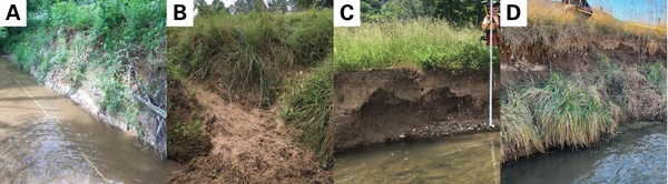
Figure 1. Types of streambank erosion: A. surface scour; B. hoof shear; C. unstable undercut; D. mass wasting.
How to Document and Quantify Sediment Volumes from Streambank Erosion
Various methods exist for documenting and quantifying streambank erosion rates through field and desktop geospatial methods. In the field, cross-sectional surveys or erosion pins are commonly used to measure bank retreat (Purvis and Fox 2016). Repeat surveys with a total station can be used to accurately measure changes in cross-section geometry. (A total station is an electronic/optical survey instrument that measures angles and distances simultaneously.) Erosion pins can be installed horizontally into the bank at specified intervals. Both methods rely on stable control points to provide an accurate estimate of erosion rates. A comparison of methods by Myers et al. (2019) reported that it can be difficult to capture the spatial variability of streambank erosion with erosion pins. Both methods are better suited for smaller watersheds (less than 100 square miles), where the stream can be easily waded without safety concerns. The erosion estimates from these methods are also representative only of changes at the specific cross-section and are unable to capture episodic streambank erosion (Purvis and Fox 2016).
Aerial imagery analysis is a geospatial method that can be used to quantify streambank retreat (Purvis and Fox 2016). Streambank locations are manually traced through visual analysis of aerial photos using GIS software. The banks are traced for each time period when photos are available and then compared to quantify streambank retreat. This method is more appropriate for larger waterways, when photos with good resolution are available, and for erosion studies focused on longer time periods. The manual delineation of streambanks is time-consuming and leaves room for subjectivity, which limits the ability to replicate studies (Williams et al. 2020).
Williams et al. (2020) developed an automated Python and ArcPy model called Aerial Imagery Migration Model (AIMM) to produce migration maps and sediment volumes from streambank erosion. This method requires significantly less time than manual delineations, but the accuracy of the results will depend on the quality of the aerial photos and resolution of the digital elevation model (DEM).
LiDAR (light detection and ranging) surveys are another method that has been used to quantify streambank erosion rates. Differences in LiDAR-derived DEMs are used to detect geomorphic changes (Schaffrath, Belmont, and Wheaton 2015). LiDAR uses point clouds to capture three-dimensional surfaces from laser-based measurements (Myers, Rediske, and McNair 2019). LiDAR data accuracy can be affected by dense vegetation. The chance the laser pulse will reach the ground is inversely proportional to the vegetation density.
The method best suited for a project will depend on the overall goal, scope, time frame, and budget as well as the accuracy and resolution needed and the method that is feasible to sustain throughout the testing period. If you are focused on immediate anthropogenic impacts, shorter studies are acceptable.
Table 1 provides a comparison of scale, resolution, and limitations for several methods for measuring streambank erosion.
| Method | Resolution | Spatial Scale [a] | Temporal Scale [b] | Limitations |
|---|---|---|---|---|
| Erosion Pins | 3 mm [3] | Small [2,3,4] | Short (months or years) or long [2,4] | Captures erosion at specific locations |
| Total Stations | ≥ 2 cm [1] | Small [2] | Short (months or years) or long [3,4] | Accuracy affected by point density; better at capturing specific locations |
| Aerial Imagery | Dependent on imagery resolution [3,4] |
Small (excluding headwaters) or large [3,4]
|
Short (2–5 years) or long [3,4]
|
Bank migration rates must be greater than photo resolution; exclude bars Cannot be used in forested or other highly vegetated areas Assumes vertical banks [4] |
| AIMM: Aerial Imagery | 1 m [4] | |||
| AIMM: DEM | 2 m |
[a] Small scale: watersheds < 100 mi2; Large scale: watersheds > 100 mi2 ↲
[b] Short term: < 5 years; Long term: > 10 years ↲
[1] (Booth and Henshaw 2001) ↲
[2] (Myers, Rediske, and McNair 2019)
[3] (Purvis and Fox 2016)
[4] (Williams et al. 2020) ↲
Field Methods
Surveying
Streambank erosion rates can be calculated using measured cross-sectional and top of bank (TOB) surveys with a total station. The use of total station surveys works well on both vegetated and bare banks (Myers, Rediske, and McNair 2019).
Below is a list of the equipment recommended for establishing and surveying permanent cross-sections:
Establish Permanent Cross-Sections:
-
Wood survey stakes
-
Rebar pins (#3 or #4)
-
Plastic rebar caps
-
GPS to record location of rebar pins
Surveying Permanent Cross-Sections and TOB:
-
Total station
-
Survey tripod
-
Notebook or handheld device to record survey data
-
Pins and clips
-
Tape measure
-
Survey rod
-
Prism
Establish and Resurvey Permanent Cross-Sections
It is important to select sites that are actively eroding to capture a measurable change in the streambank.
-
Stretch a tape measure across the stream perpendicular to the eroding bank (Figure 2). Drive a rebar pin into the ground on both sides of the stream along the alignment. The rebar pins should be far enough back from the banks that the pins will not be exposed or lost if the bank erodes. Carefully tap a plastic cap on top of the pin and ensure the cap is flush with the ground. Drive a wood stake into the ground behind each pin to easily locate the pins in the future. If the total station cannot be set up on one of the cross-section pins, sink a third rebar pin and plastic cap into the ground to establish a benchmark for the total station. Select a location where the entire cross-section is visible, but not too close so as not to hamper data collection using the total station. This location should ideally be on top of the streambank that is opposite of the most severe erosion (usually set up on the inside of the bend as most erosion occurs on the outside of bends).
-
Use temporary pins and clips to affix the tape measure between the permanent pin locations. The tape will serve as a guide when surveying the cross-section. Ensure the tape is secure and taut. The tape does not need to be level as the total station captures both the station and elevation along the cross-section.
-
Collect survey measurements at each point of inflection along the cross-section following the tape. Fewer data points are required on the floodplain. More points should be collected along each side of the bank to accurately capture the shape of the bank. If the channel is actively incising, more points should be collected along the bed. Carefully name all survey points in the survey notes or handheld device and take pictures to document the cross-section, especially the eroding banks.
Undercut Banks
Undercut banks are difficult to survey and are often eliminated from studies (Myers, Rediske, and McNair 2019; Williams et al. 2020). Two methods can be used to capture undercut banks depending on the position of the total station.
-
If the total station is located on the bank opposite the undercut, the prism can be placed directly against the bank and the rod height set to 0 ft (Figure 3). Removing the prism from the rod makes it easier to position the prism at the desired location.
-
If the total station is not situated well to capture an undercut bank, measure the horizontal offset between the survey rod and point of inflection at a 90° angle (Figure 3). Notate the horizontal offset value in the point name so the station can be manually adjusted afterward.
Resurvey Period
After a period of one year, return to the site and resurvey each cross-section using the same procedures. Surveys completed one year apart will allow for the development of annual erosion rates.
Survey Eroding Top of Bank (TOB)
Streambank erosion is generally non-uniform in both the vertical and longitudinal directions. Cross-sections capture erosion at only one specific longitudinal location. Therefore, surveying the edge of the top of the eroding banks both upstream and downstream of the cross-section can capture the variability of the erosion. TOB surveyed along all eroding portions of the study reach can be used to tally the length of the stream that is eroding and to quantify reach-wide bank retreat. By capturing the TOB location during annual surveys, average lateral erosion can be calculated for each eroding meander bend or streambank segment.
TOB is located at the edge of the bank where the erosion starts and the bank drops off. It can sometimes be difficult to determine where to place the survey rod for TOB shots. Figure 4 demonstrates surveying the TOB. A point should be collected every couple of feet or often enough to capture the shape of the bank. TOB measurements are useful only at locations experiencing larger amounts of erosion, because the error rate for this measurement can be substantial.
If TOB is not surveyed, measure the length of each eroding section of the stream while in the field to facilitate calculating erosion volumes.
Soil Samples
Soil samples can be collected from the eroding streambanks and analyzed for total nitrogen (TN), total phosphorus (TP), and bulk density.
Bulk density is used to estimate sediment mass loads and TN and TP concentrations can be used to estimate nitrogen and phosphorus loads from streambank erosion. Samples should be collected at each cross-section on the eroding bank(s) during the first-year visit. If stratification is present, soil samples should be collected from each distinctive layer. Hammer a round bottomless metal cylinder (soil core sampler) into the bank (Figure 5). The edge of the cylinder should be flush with the bank. Pushing the cylinder too far into the bank can compact the soil, increasing the bulk density. Remove the cylinder and place the cylinder and the soil sample in a bag labeled with the cross-section and the bank side (left or right).
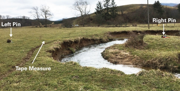
Figure 2. Set up for surveying a stream cross-section, showing pin on left and right banks and tape measure stretched between them.
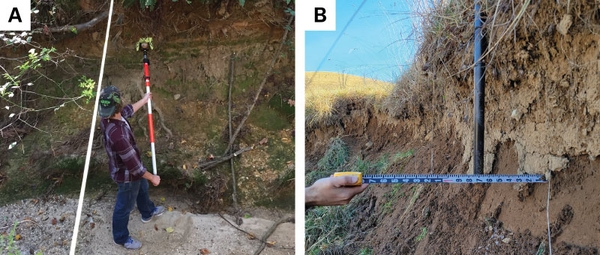
Figure 3. Methods used to survey undercut banks, including placing the prism against the streambank with 0 feet for rod height (left) and horizontal offset measurement where the bottom of the survey rod is lowered to the point of inflection and a ruler is used to measure the distance to the bank at 90° (right).
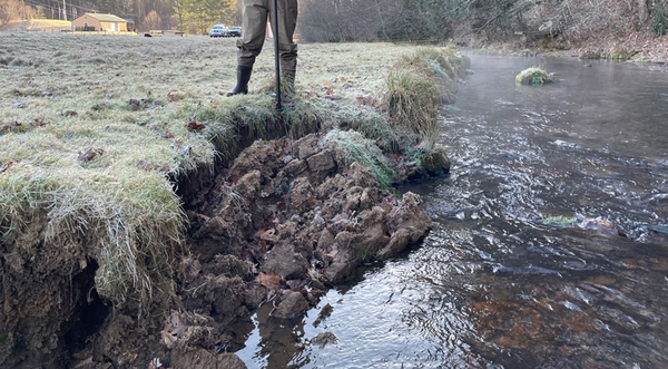
Figure 4. Example of rod placement for TOB survey along a collapsed streambank.
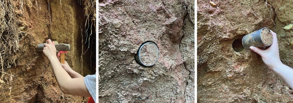
Figure 5. Collecting soil sample with sledgehammer and cylindrical metal soil core sampler.
Processing Field-Collected Data
Quantify Bank Retreat (ft/yr) from Cross-Sections
Microsoft Excel Method
In Excel, linear interpolation can be used to obtain the station of the streambank for each survey year at every 0.5 ft elevation interval between the selected top and bottom of the bank. Calculate the difference between the interpolated year 1 station and year 2 station to estimate the bank retreat at each 0.5 ft vertical interval (see Equation 1 for the left bank calculation and Equation 2 for the right bank calculation). Negative values represent erosion; positive values represent deposition.
Equation 1
Left bank retreat (ft)= Year 2 station (ft) −Year 1 station (ft)
Equation 2
Right bank retreat (ft)= Year 1 station (ft) −Year 2 station (ft)
Determine the survey error by repeating surveys at selected cross-sections during the same survey visit. The repeat surveys can be done during the first- or second-year. Eliminate any measured bank retreat less than the survey error. Both human error (for example, incorrectly setting the rod height, taking points when the rod is not completely vertical, or collecting the survey shot before the rod is in contact with the ground) and environmental conditions (for example, animal and/or human disturbance of the survey pin or freeze/thaw cycles moving the pin) can affect the accuracy of the survey data. Sum the retreat values and divide by the total number of 0.5-foot intervals along the streambank to determine the average bank retreat. You can also identify the maximum and minimum erosion rate for each bank. Example calculations are provided in Appendix A.
AutoCAD Method
Copy and paste the overlaid cross-sections from Excel into AutoCAD. Ensure the scale is correct. Use the polyline tool to trace the area of the cross-section, making sure to not go beyond the selected top and bottom of the bank to form a polygon. Use properties to get the area of the polygon and divide by the bank height to get an average bank retreat (ft/yr). Ensure that the traced polygon represents erosion and not deposition.
Quantify Reach-Wide Volumes of Eroded Material (ft3/yr)
Cross-Section Surveys
To estimate a volume of eroded material (ft3/yr), the bank retreat (ft/yr) calculated from the cross-section surveys is multiplied by the bank height (ft) and length of eroding section (ft). The bank height can either be measured in the field or estimated from cross-section surveys. The length of the eroding section should have been marked in the field with TOB survey or measured in the field. We recommend calculating the minimum, average, and maximum bank retreat values from the cross-section surveys to account for the uncertainty in measuring and quantifying streambank erosion rates and associated volumes.
TOB Surveys
The volume of soil eroded can also be estimated using TOB surveys. Figure 6 shows an overlay of two years of the TOB survey for an eroding meander bend. From the figure you can see the bank retreat is more severe downstream of where the cross-section is located.
The lateral area of erosion can be calculated by comparing the two TOB measurements, following a very similar method to the aerial imagery analysis laid out by Purvis and Fox (2016). The area of erosion can then be multiplied by the height of the streambank obtained from the field measurement of the cross-section to generate a volume of total erosion that has occurred during the time between surveys. Procedures for the TOB overlay comparison and volumetric calculations using ArcGIS Pro or ArcMap are provided in Appendix B.
Test Soil Samples for Bulk Density, TN, and TP
Collected soil samples should be analyzed for bulk density, TN, and TP in a laboratory. The laboratory test used to gauge nutrient concentrations should measure the soil-attached nutrients that can be lost to the receiving water and not what is available to plants. A recommended methodology for measuring TN is the APHA 4500 Norg B methodology, and for TP, the APHA 4500-P F methodology. Bulk density can be measured using the ASTM D 7263 method (D18 Committee 2021). In addition, the Chesapeake Bay Program recommends measuring the total-sorbed P (EPA Method 3051 + 6010) (US EPA 1986) and total N combustion testing (Bremner 2018).
Calculate Annual Sediment and Nutrient Loads
To estimate the eroded sediment volume (cubic feet), multiply the measured bank height by the bank retreat and length of the associated stream segment. To present this value in tons of sediment per year, convert the eroded volume to cubic cm and then multiply it by the average bulk density (g/cm3) and convert from grams to tons. The average bulk density is obtained from the laboratory analysis of the soil samples taken at each cross-section. Bulk density can also be estimated from published soil surveys of the area. Divide the sediment load by the centerline length of the stream to get an erosion rate per linear foot of stream channel (Walter, Merritts, and Rahnis 2007; Wegmann et al. 2013). Or divide by the length of the eroding bank to calculate a sediment load for a specific segment of streambank.
If time or budget does not allow for conducting repeat cross-section surveys, then streambank retreat rates can be estimated using erosion curves based on Bank Erosion Hazard Index (BEHI) and Near-Bank Stress (NBS) assessments following protocols developed by Anne Arundel County, Maryland (Starr 2009). The Chesapeake Stormwater Network also provides detailed standard BEHI methods (Atland et al. 2020). BEHI and NBS assessments must be performed for each eroding streambank.
Minimum, average, and maximum bank retreat values calculated from the measured cross-sections can be applied to estimate a range of sediment and nutrient loads from streambanks using the steps outlined below:
- Calculate the volume of erosion (ft3/yr):
- Multiply the length of the eroded bank at each cross-section by the average measured bank retreat and measured bank height.
- For eroding banks without cross-sections, multiply the area of erosion from TOB surveys by the measured bank height.
- To quantify the volume of erosion for the entire reach, sum the total volume of sediment for all eroded streambanks with measured cross-sections and TOB surveys.
- Calculate the total load of sediment (tons/yr). Multiply the volume of sediment by the average bulk density of the soil in the study area. Be sure all units match.
- Convert volume from cubic feet to cubic cm.
- Multiple volume in cubic cm by average bulk density (g/cm3).
- Convert grams (g) to US tons (tons).
- Estimate the TN and TP loads.
- Multiply the load of sediment (grams) by the average measured TN and TP concentrations (mg/g of dry weight).
- Convert milligrams (mg) to pounds (lb).
- Divide the total load in pounds of TN and TP by the watershed area to compare nutrient loads between various stream reaches and study locations.
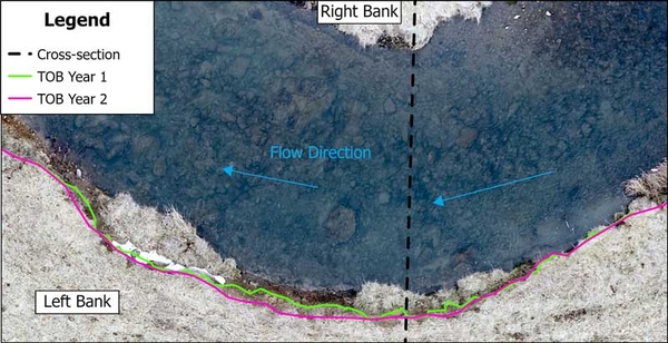
Figure 6. TOB surveys in ArcGIS.
Desktop Method—Aerial Imagery Analysis
Reach-wide erosion rates and sediment loads can be estimated using aerial imagery analysis. As previously mentioned, this method is suitable only for sites with minimal tree cover so the TOB is clearly visible. It is best to select images over a longer temporal scale to ensure that the amount of erosion measured exceeds the resolution of the images. Capturing aerial images of a specific study site with a drone is highly recommended, as it will provide better-quality images compared to images downloaded from public sources. These images must be scaled and orthorectified to calculate accurate measurements (Rocchini and Di Rita 2005).
In a GIS software, polylines are drawn along the TOB, based on visual interpretation of the edge of the streambank location. The polylines representing the streambanks are compared between years to quantify past erosion rates, following methods outlined by Purvis and Fox (2016). User error for this method can be estimated by repeating the delineation of several streambanks and calculating the percent difference in the area of erosion between delineations. The erosion difference can then be standardized by the linear feet of stream delineated (ft2/ft/yr). We recommend selecting a bank that is easy to delineate (minimal obstruction of the TOB) and one that is more difficult (obstruction due to shadows and overhanging vegetation) to capture the range of error.
The volume of sediment is estimated by multiplying the height of the streambank by the area of erosion. The bank height could be estimated from a digital elevation model (DEM) or measured in the field. Figure 7 depicts the key steps of the analysis. To get volume of erosion per linear foot of stream per year (ft3/linear ft/yr), divide the erosional volume of each bank by the length of the bank based on the bank line from year 1 and then divide by the number of years between images. Additional details outlining this method are provided in Appendix C.
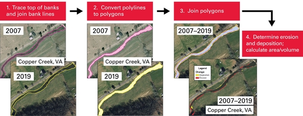
Figure 7. Main steps for aerial imagery analysis.
References
Atkins, Rachel M., Karl W. Wegmann, and Del Wayne R. Bohnenstiehl. 2023. “Channel Head Response to Anthropogenic Landscape Modification: A Case Study from the North Carolina Piedmont, USA, with Implications for Water Quality.” Earth Surface Processes and Landforms 48 (2): 433–51.
Atland, Drew, Joe Berg, Josh Burch, Reid Cook, Lisa Fraley-McNeeal, Matt Meyers, Josh Running, et al. 2020. “Consensus Recommendations for Improving the Application of the Prevented Sediment Protocol for Urban Stream Restoration Projects Built for Pollutant Removal Credit.” Chesapeake Stormwater Network.
Booth, Derek B., and Patricia C. Henshaw. 2001. “Rates of Channel Erosion in Small Urban Streams.” In Water Science and Application, edited by Mark S. Wigmosta and Stephen J. Burges, 2:17–38. Washington, D. C.: American Geophysical Union.
Bremner, J. M. 2018. “Nitrogen-Total.” In Methods of Soil Analysis: Part 3 Chemical Methods, edited by D.L. Sparks, A.L. Page, P.A. Helmke, R.H. Loeppert, P. N. Soltanpour, M. A. Tabatabai, C. T. Johnston, and M. E. Sumner, 1085–1121. SSSA Book Series. Madison, WI, USA: Soil Science Society of America, American Society of Agronomy.
D18 Committee. 2021. “Test Methods for Laboratory Determination of Density (Unit Weight) of Soil Specimens.” ASTM International. https://doi.org/10.1520/D7263-21.
DWER. 2000. “Sediment in Streams.” Water and Rivers Commission. 2000.
Florsheim, Joan L., Jeffrey F. Mount, and Anne Chin. 2008. “Bank Erosion as a Desirable Attribute of Rivers.” BioScience 58 (6): 519–29.
Gage, Maury S., Aaron Spivak, and Christopher J. Paradise. 2004. “Effects of Land Use and Disturbance on Benthic Insects in Headwater Streams Draining Small Watersheds North of Charlotte, NC.” Southeastern Naturalist 3 (2): 345–58.
Hopkins, Kristina G., Nathaniel B. Morse, Daniel J. Bain, Neil D. Bettez, Nancy B. Grimm, Jennifer L. Morse, Monica M. Palta, William D. Shuster, Anika R. Bratt, and Amanda K. Suchy. 2015. “Assessment of Regional Variation in Streamflow Responses to Urbanization and the Persistence of Physiography.” Environmental Science & Technology 49 (5): 2724–32.
Hupp, Cliff R., Gregory B. Noe, Edward R. Schenk, and Adam J. Benthem. 2013. “Recent and Historic Sediment Dynamics along Difficult Run, a Suburban Virginia Piedmont Stream.” Geomorphology 180–181 (January): 156–69.
Lammers, Roderick W., and Brian P. Bledsoe. 2019. “Quantifying Pollutant Loading from Channel Sources: Watershed-Scale Application of the River Erosion Model.” Journal of Environmental Management 234 (March): 104–14.
Myers, Daniel T., Richard R. Rediske, and James N. McNair. 2019. “Measuring Streambank Erosion: A Comparison of Erosion Pins, Total Station, and Terrestrial Laser Scanner.” Water 11 (9): 1846.
Noe, G B, K G Hopkins, P R Claggett, E R Schenk, M J Metes, L Ahmed, T R Doody, and C R Hupp. 2022. “Streambank and Floodplain Geomorphic Change and Contribution to Watershed Material Budgets.” Environmental Research Letters 17 (6): 064015.
Palmer, Jason A., Keith E. Schilling, Thomas M. Isenhart, Richard C. Schultz, and Mark D. Tomer. 2014. “Streambank Erosion Rates and Loads within a Single Watershed: Bridging the Gap between Temporal and Spatial Scales.” Geomorphology 209 (March): 66–78.
Paterson, Robert G., Michael I. Luger, Raymond J. Burby, Edward J. Kaiser, H. Rooney Malcom, and Alicia C. Beard. 1993. “Costs and Benefits of Urban Erosion and Sediment Control: The North Carolina Experience.” Environmental Management 17 (2): 167–78.
Purvis, Rebecca A., and Garey A. Fox. 2016. “Streambank Sediment Loading Rates at the Watershed Scale and the Benefit of Riparian Protection: Streambank Sediment Loading Rates at the Watershed Scale.” Earth Surface Processes and Landforms 41 (10): 1327–36.
Rocchini, D., and A. Di Rita. 2005. “Relief Effects on Aerial Photos Geometric Correction.” Applied Geography 25 (2): 159–68.
Russell, Kathryn L., Geoff J. Vietz, and Tim D. Fletcher. 2017. “Global Sediment Yields from Urban and Urbanizing Watersheds.” Earth-Science Reviews 168 (May): 73–80.
Russell, Kathryn L., Geoff J. Vietz, and Tim D. Fletcher. 2019. “A Suburban Sediment Budget: Coarse‐grained Sediment Flux through Hillslopes, Stormwater Systems and Streams.” Earth Surface Processes and Landforms 44 (13): 2600–2614. h
Schaffrath, Keelin R., Patrick Belmont, and Joseph M. Wheaton. 2015. “Landscape-Scale Geomorphic Change Detection: Quantifying Spatially Variable Uncertainty and Circumventing Legacy Data Issues.” Geomorphology 250 (December): 334–48.
Simon, Andrew. 1989. “A Model of Channel Response in Disturbed Alluvial Channels.” Earth Surface Processes and Landforms 14 (1): 11–26.
Simon, Andrew, and Massimo Rinaldi. 2006. “Disturbance, Stream Incision, and Channel Evolution: The Roles of Excess Transport Capacity and Boundary Materials in Controlling Channel Response.” Geomorphology 79 (3–4): 361–83.
Starr, Richard. 2009. “Stream Assessment Protocol Anne Arundel County, Maryland.” U.S. Fish and Wildlife Service.
Stott, Tim. 1997. “A Comparison of Stream Bank Erosion Processes on Forested and Moorland Streams in the Balquhidder Catchments, Central Scotland.” Earthh Surface Processes and Landforms 22 (4): 383–99.
US EPA. 1986. “Test Methods for Evaluating Solid Waste.” SW-846. Springfield, VA.
US EPA. 2015. “A Compilation of Cost Data Associated with the Impacts and Control of Nutrient Pollution.” Office of Water, EPA 820-F-15-096. US Environmental Protection Agency.
US EPA. 2017. “National Water Quality Inventory: Report to Congress.” 841-R-16–011.
Walter, Robert, Dorothy Merritts, and Mike Rahnis. 2007. “Estimating Volume, Nutrient Content, and Rates of Stream Bank Erosion of Legacy Sediment in the Piedmont and Valley and Ridge Physiographic Provinces, Southeastern and Central PA.” Report to the Pennsylvania Department of Environmental Protection, Lancaster, Pennsylvania.
Wegmann, Karl W., Christopher L. Osburn, Robert Q. Lewis, Peszlen, and Helena Mitasova. 2013. “Legacy Sediments and Stream Water Quality: Estimating Volume, Nutrient Content, and Stream Bank Erosion in 303(d)-Impaired Waterways of the North Carolina Piedmont.” 435. Water Resources Research Institute of the University of North Carolina.
Williams, Forrest, Peter Moore, Thomas Isenhart, and Mark Tomer. 2020. “Automated Measurement of Eroding Streambank Volume from High-Resolution Aerial Imagery and Terrain Analysis.” Geomorphology 367 (October): 107313.
Wohl, Ellen, Brian P. Bledsoe, Robert B. Jacobson, N. LeRoy Poff, Sara L. Rathburn, David M. Walters, and Andrew C. Wilcox. 2015. “The Natural Sediment Regime in Rivers: Broadening the Foundation for Ecosystem Management.” BioScience 65 (4): 358–71.
Appendix A. Procedure to Quantify Streambank Retreat
Two surveys of each cross-section collected at different time periods can be used to determine the rate of streambank retreat. Bank retreat is calculated separately for the right and left banks. Any point bars or stream banks that exhibit deposition rather than erosion should be excluded from the analysis.
- Prepare a graphical overlay of the cross-section data for both years using Excel or other software with graphing capability.
- Visually identify the “vertical” portion of the bank using the overlaid cross-section survey plot (Figure A.1) and pictures of the cross-section (Figure A.2). Select the TOB elevation as the lower of the two surveys; select the toe of bank elevation as the higher of the two surveys (Figure A.1), being sure to exclude any slumped material that could skew the results.
- Interpolate the station of the streambank for Year 1 and Year 2 at every 0.5 ft vertical elevation interval between the selected top and toe of bank elevation.
- Calculate the bank retreat by subtracting the stations. Negative values represent erosion; positive values represent deposition.
- Left bank: Year 2 − Year 1
- Right bank: Year 1 − Year 2
- Set all values representing deposition to 0 ft/yr bank retreat.
- Any horizontal distance values between the Year 1 and Year 2 stations that are less than the margin of error should be set to 0 ft/yr bank retreat.
- Calculate the maximum, average, and minimum bank retreat (ft/yr) for each bank.
- Calculate the area of eroded material:
- Area of eroded material (ft2/yr) = Bank retreat (ft/yr) × Bank height (ft)
- The bank height is the difference between the top of bank and toe of bank elevations.
- Determine the length of the eroding stream bank for the cross-section using ArcGIS.
- Calculate the volume of eroded material:
-
Volume of eroded material (ft3/yr) = Area of eroded material (ft2/yr) × Length of stream bank (ft)
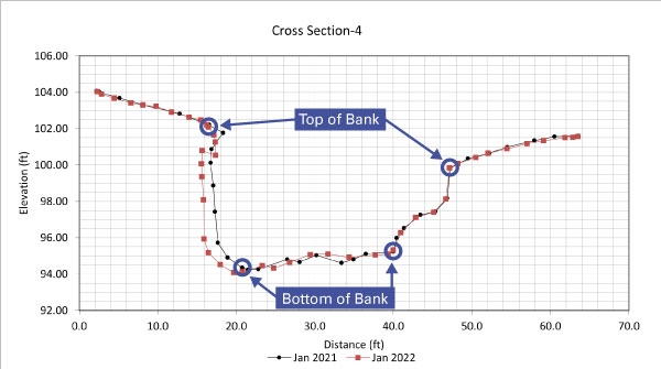
Figure A.1. Example of plotted overlays of cross-section data from two surveys with selection of top and bottom of bank elevations.
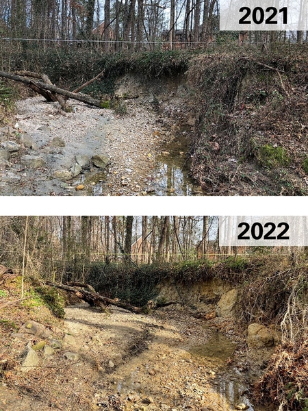
Figure A.2. Pictures of the stream cross-section taken during surveys.
Appendix B. Top of Bank Survey Procedure
The following steps are based on using ArcGIS software. Repeat the steps for each cross-section.
- Import the Year 1 and Year 2 TOB surveys.
- Define the coordinate system to enable using ArcGIS tools.
- Create a new feature class for construction lines.
- Draw construction lines at the beginning and end of the TOB surveys, making sure to intersect both TOB lines. Place the construction lines at the end of the shorter survey (Figure B.1).
- Create a polygon from the polylines (Figure B.2).
- Join Year 1 and Year 2 polygons.
- Categorize and label each polygon section as either erosion or deposition (Figure B.3).
- Separate the multipart polygon for erosion and deposition into single polygons.
- Calculate the area of each polygon.
- Add fields to the attribute table for bank height and volume. Bank height can be obtained from field measurements or DEM data.
- Calculate the volume of eroded material:
Volume of eroded material (ft3/yr) = Area of eroded material (ft2/yr) × Length of stream bank (ft)
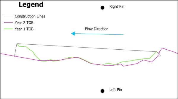
Figure B.1. Example of drawing construction lines in relation to TOB surveys in ArcGIS.
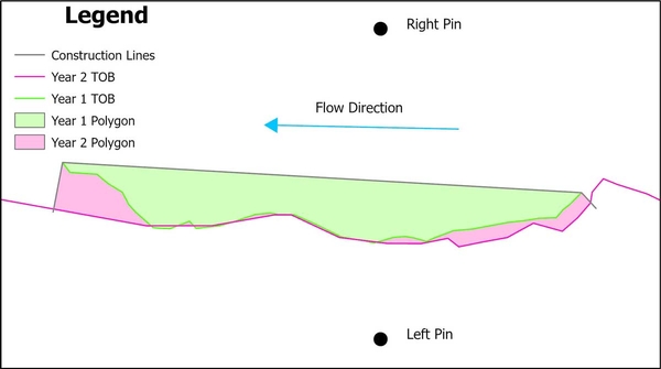
Figure B.2. Year 1 and Year 2 polygons created from TOB and construction lines.
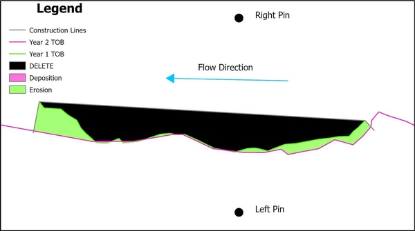
Figure B.3. This shows the Year1_Year2_change polygon and which sections of the polygon are erosion (green), which are deposition (pink), and which should be deleted (black).
Appendix C. Aerial Imagery Analysis Procedure
The following steps are based on using ArcGIS software.
- Create a feature class for Year 1 and Year 2. Be sure to match it to the coordinate system of the image.
- Trace the top of bank from the start and end of the study reach for Year 1. Select a scale that best fits with the resolution of the image. For imagery with 1 ft resolution, 1:850 scale was used. For 0.05 ft resolution, a scale of 1:200 is recommended.
- Adjust vertices as needed when zooming into 1:500 and zooming out to 1:1,000 to ensure accuracy, if using 1:850 scale. Adjust the scales as appropriate for the resolution of images used.
- Draw construction lines at the beginning and end of the study reach, making sure to intersect the bank lines.
- Repeat Steps 2 through 4 for Year 2.
- Create a polygon from polylines for Year 1 and Year 2.
- Join Year 1 and Year 2 polygons.
- Categorize and label each polygon sections as either erosion or deposition.
- Delete any extraneous polygons at the beginning and end of the study reach created from the boundaries.
- Separate the multipart polygon for erosion and deposition into single polygons.
Steps 11 to 17 are applicable only if there is no overlap between the Year 1 and Year 2 channel due to large shifts in the stream (Figure C.1). Without these steps, the gap between the new and old channel would be excluded from the total erosion and deposition amounts.
- Create a copy of bank lines where there is no overlap.
- Split the Year 1 bank lines so there are separate segments for just the part with no overlap. Repeat for Year 2.
- Create a new polygon that represents both erosion and deposition from the newly segmented bank lines (Figure C.2).
- Copy the polygon made in step 13 and paste in the polygon layer made in step 7 (Figure C.2).
- Merge the copied polygon with the adjacent deposition polygon.
- Repeat steps 13 and 14.
- Merge the copied polygon with the adjacent erosion polygon.
- Calculate the area of each polygon.
- Add fields to the attribute table for bank height and volume. Bank height can be obtained from field measurements or DEM data. It is recommended to break the reach into segments based on changes in bank height.
- Calculate the volume of eroded material:
Volume of eroded material (ft3/yr) = Area of eroded material (ft2/yr) × Length of stream bank (ft)
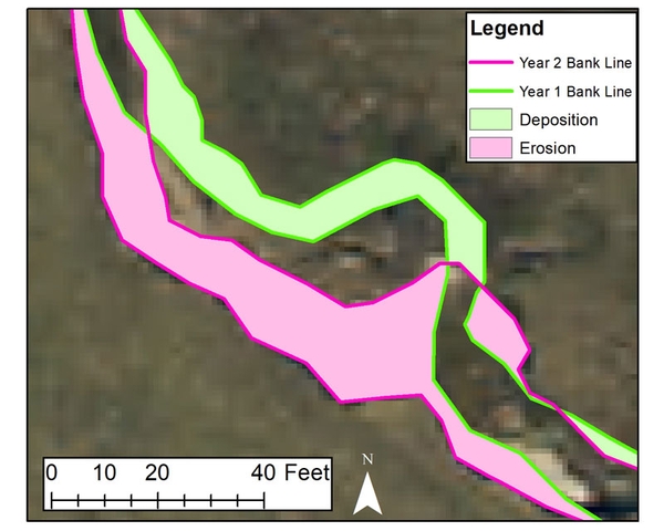
Figure C.1. Example of no overlap between old and new channels.
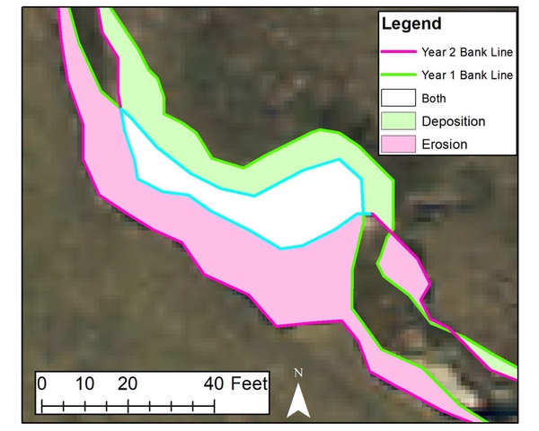
Figure C.2. Polygon between old and new channels that represents both deposition and erosion.
Publication date: June 6, 2024
AG-956
N.C. Cooperative Extension prohibits discrimination and harassment regardless of age, color, disability, family and marital status, gender identity, national origin, political beliefs, race, religion, sex (including pregnancy), sexual orientation and veteran status.
